Observed vs. predicted plots

Generates plots comparing predictions with observations.

pred.plot(pred, obs, ...)

# S3 method for default
pred.plot(
  pred,
  obs,
  xlab = "Predicted",
  ylab = "Observed",
  lm.fit = TRUE,
  lowess = TRUE,
  ...
)

# S3 method for factor
pred.plot(
  pred,
  obs,
  type = c("frec", "perc", "cperc"),
  xlab = "Observed",
  ylab = NULL,
  legend.title = "Predicted",
  label.bars = TRUE,
  ...
)

Arguments

pred

a numeric vector with the predicted values.

obs

a numeric vector with the observed values.

...

additional graphical parameters or further arguments passed to other methods (e.g. to RcmdrMisc::Barplot()).

xlab

a title for the x axis.

ylab

a title for the y axis.

lm.fit

logical indicating if a lm fit is added to the plot.

lowess

logical indicating if a lowess smooth is added to the plot.

type

types of the desired plots. Any combination of the following values is possible: "frec" for frequencies, "perc" for percentages or "cperc" for conditional percentages.

legend.title

a title for the legend.

label.bars

if TRUE (the default) show values of frequencies or percents in the bars.

Value

The default method invisibly returns the fitted linear model if lm.fit == TRUE.

pred.plot.factor() invisibly returns the horizontal coordinates of the centers of the bars.

Details

The default method draws a scatter plot of the observed values against the predicted values.

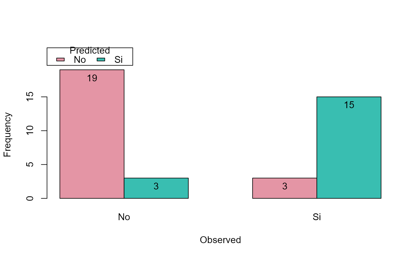
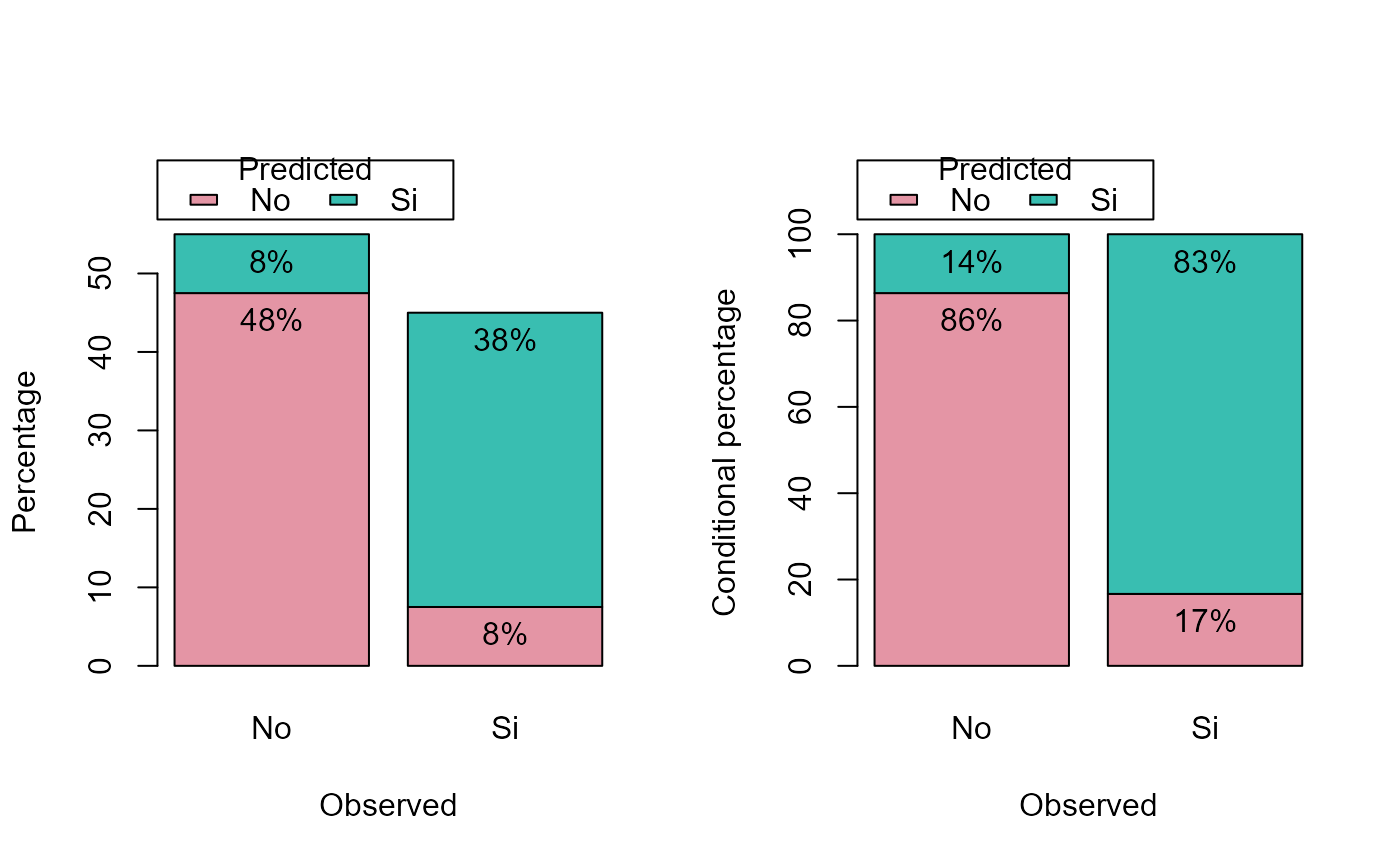
pred.plot.factor() creates bar plots representing frequencies, percentages or conditional percentages of pred within levels of obs. This method is a front end to RcmdrMisc::Barplot().

See also

accuracy()

Examples

set.seed(1)
nobs <- nrow(hbat)
itrain <- sample(nobs, 0.8 * nobs)
train <- hbat[itrain, ]
test <- hbat[-itrain, ]

# Regression
fit <- lm(fidelida ~ velocida + calidadp, data = train)
pred <- predict(fit, newdata = test)
obs <- test$fidelida
res <- pred.plot(pred, obs)

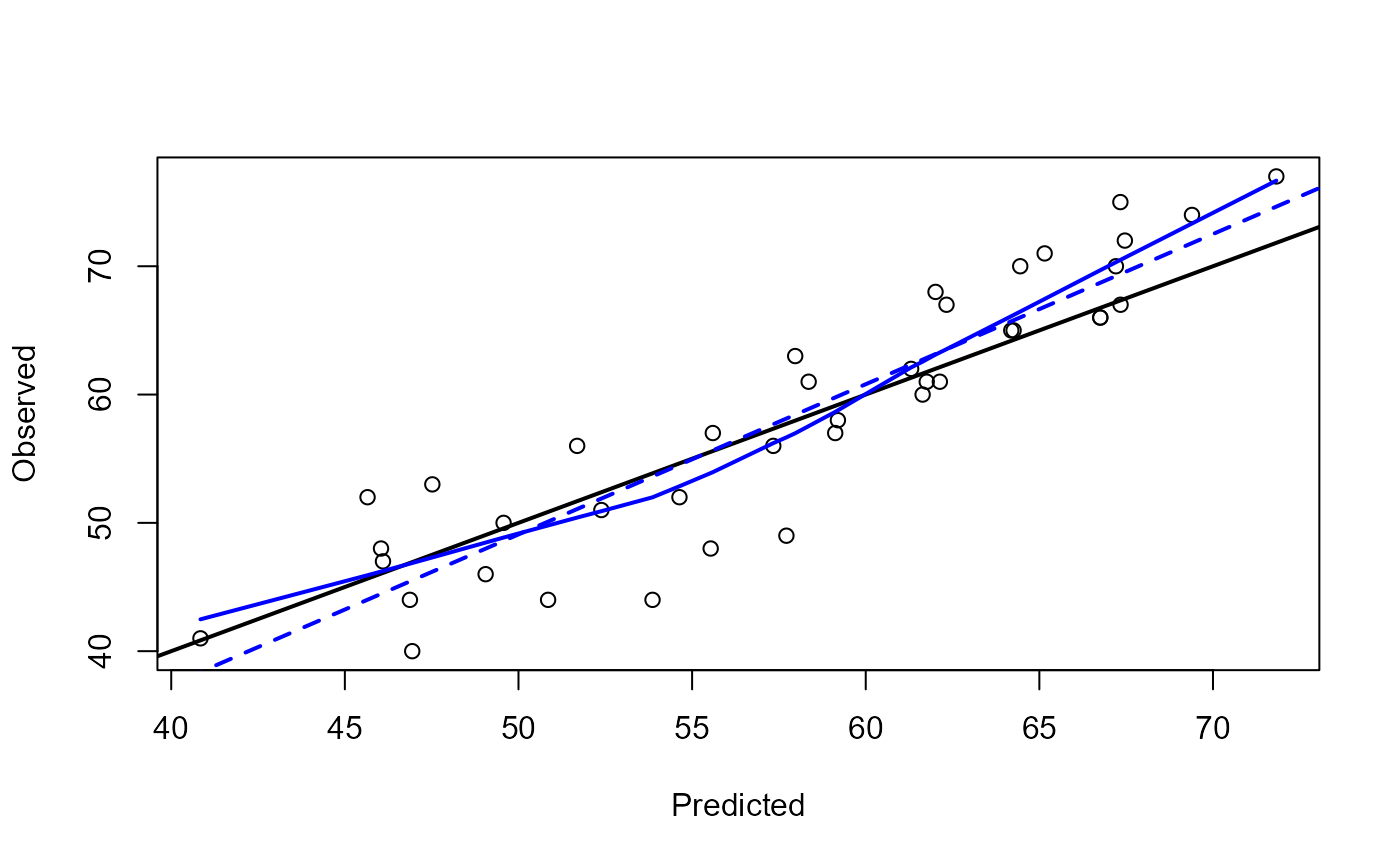summary(res)
#> 
#> Call:
#> lm(formula = obs ~ pred)
#> 
#> Residuals:
#>     Min      1Q  Median      3Q     Max 
#> -9.6170 -2.4273 -0.5227  2.8353  7.9903 
#> 
#> Coefficients:
#>             Estimate Std. Error t value Pr(>|t|)    
#> (Intercept) -9.43398    4.92829  -1.914   0.0631 .  
#> pred         1.17064    0.08433  13.881   <2e-16 ***
#> ---
#> Signif. codes:  0 '***' 0.001 '**' 0.01 '*' 0.05 '.' 0.1 ' ' 1
#> 
#> Residual standard error: 4.206 on 38 degrees of freedom
#> Multiple R-squared:  0.8353,	Adjusted R-squared:  0.8309 
#> F-statistic: 192.7 on 1 and 38 DF,  p-value: < 2.2e-16
#> 

# Classification
fit2 <- glm(alianza ~ velocida + calidadp, family = binomial, data = train)
obs <- test$alianza
p.est <- predict(fit2, type = "response", newdata = test)
pred <- factor(p.est > 0.5, labels = levels(obs))
pred.plot(pred, obs, type = "frec", style = "parallel")

old.par <- par(mfrow = c(1, 2))
pred.plot(pred, obs, type = c("perc", "cperc"))

par(old.par)