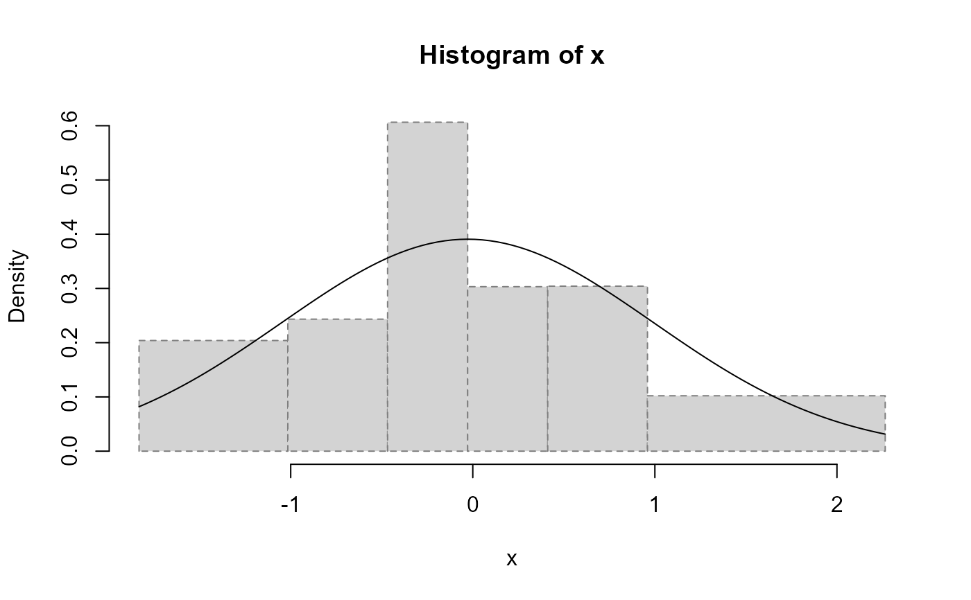
Performs the chi-squared goodness-of-fit test for a continuous distribution by grouping data into bins (also called intervals, classes or cells) with equal probabilities under the null hypothesis.
Arguments
- x
numeric vector containing the observed values.
- distribution
character string naming a continuous distribution, such as "norm" or "unif" (the cumulative distribution
p<distribution>()and quantileq<distribution>()functions must exist).- nclass
number of bins.
- output
logical; if
TRUEan histogram is plotted and a table with the results for each class is printed.- nestpar
number of estimated parameters (composite null hypothesis).
- ...
parameters of the distribution (specified by
distribution).
Value
A list with class "htest" containing the following components:
- statistic
the value the chi-squared test statistic.
- parameter
the degrees of freedom of the approximate chi-squared distribution of the test statistic.
- p.value
the p-value for the test.
- method
a character string indicating the type of test performed.
- data.name
a character string with the actual
xargument name.- classes
a character vector with the class labels.
- observed
the observed counts.
- expected
the expected counts under the null hypothesis.
- residuals
the Pearson residuals,
(observed - expected) / sqrt(expected).
See also
Examples
nx <- 30
x <- rnorm(nx)
chisq.cont.test(x, distribution = "norm", nestpar = 2,
                mean = mean(x), sd = sqrt((nx - 1) / nx) * sd(x))

#>
#> Pearson's Chi-squared test table
#>                     classes observed expected  residuals
#> 1 (-1.83297059,-1.01588461]        5        5  0.0000000
#> 2 (-1.01588461,-0.46797368]        4        5 -0.4472136
#> 3 (-0.46797368,-0.02824437]        8        5  1.3416408
#> 4 (-0.02824437, 0.41148493]        4        5 -0.4472136
#> 5 ( 0.41148493, 0.95939586]        5        5  0.0000000
#> 6 ( 0.95939586, 2.26507865]        4        5 -0.4472136
#>
#> 	Pearson's Chi-squared test
#>
#> data:  x
#> X-squared = 2.4, df = 3, p-value = 0.4936
#>
#>
#> Pearson's Chi-squared test table
#> classes observed expected residuals
#> 1 (-1.83297059,-1.01588461] 5 5 0.0000000
#> 2 (-1.01588461,-0.46797368] 4 5 -0.4472136
#> 3 (-0.46797368,-0.02824437] 8 5 1.3416408
#> 4 (-0.02824437, 0.41148493] 4 5 -0.4472136
#> 5 ( 0.41148493, 0.95939586] 5 5 0.0000000
#> 6 ( 0.95939586, 2.26507865] 4 5 -0.4472136
#>
#> Pearson's Chi-squared test
#>
#> data: x
#> X-squared = 2.4, df = 3, p-value = 0.4936
#>