Density, distribution function, quantile function and random generation for
the double-exponential distribution with rate rate.
ddexp(x, rate = 1)

pdexp(q, rate = 1)

qdexp(p, rate = 1)

rdexp(n = 1000, rate = 1)
Arguments
- x, q
vector of quantiles.
- rate
vector of rates.
- p
vector of probabilities.
- n
number of observations. If length(n) > 1, the length is taken to be the number required.
Value
ddexp() gives the density, pdexp() gives the distribution function,
qdexp() gives the quantile function, and rdexp() generates random deviates.
Details
If rate is not specified, it assumes the default value of 1.
The double-exponential distribution with rate \(\lambda\) has density $$f(x) =\frac{\lambda}{2}e^{-\lambda | x |}$$ for \(x \in \mathbb{R}\). The cummulative distribution is: $$F(x) = \int_{-\infty}^{x}f(t) dt =\left\{ \begin{array}{ll} \frac{1}{2}e^{\lambda x} & \text{if } x < 0\\ 1-\frac{1}{2}e^{-\lambda x} & \text{if } x \geq 0 \end{array} \ \right.$$ The inverse cumulative distribution function is given by $$F^{-1}(p) = - \operatorname{sign}(p-0.5)\frac{\ln(1 - 2 | p - 0.5 | )} {\lambda}.$$
See also
Examples
set.seed(54321)
rate <- 2
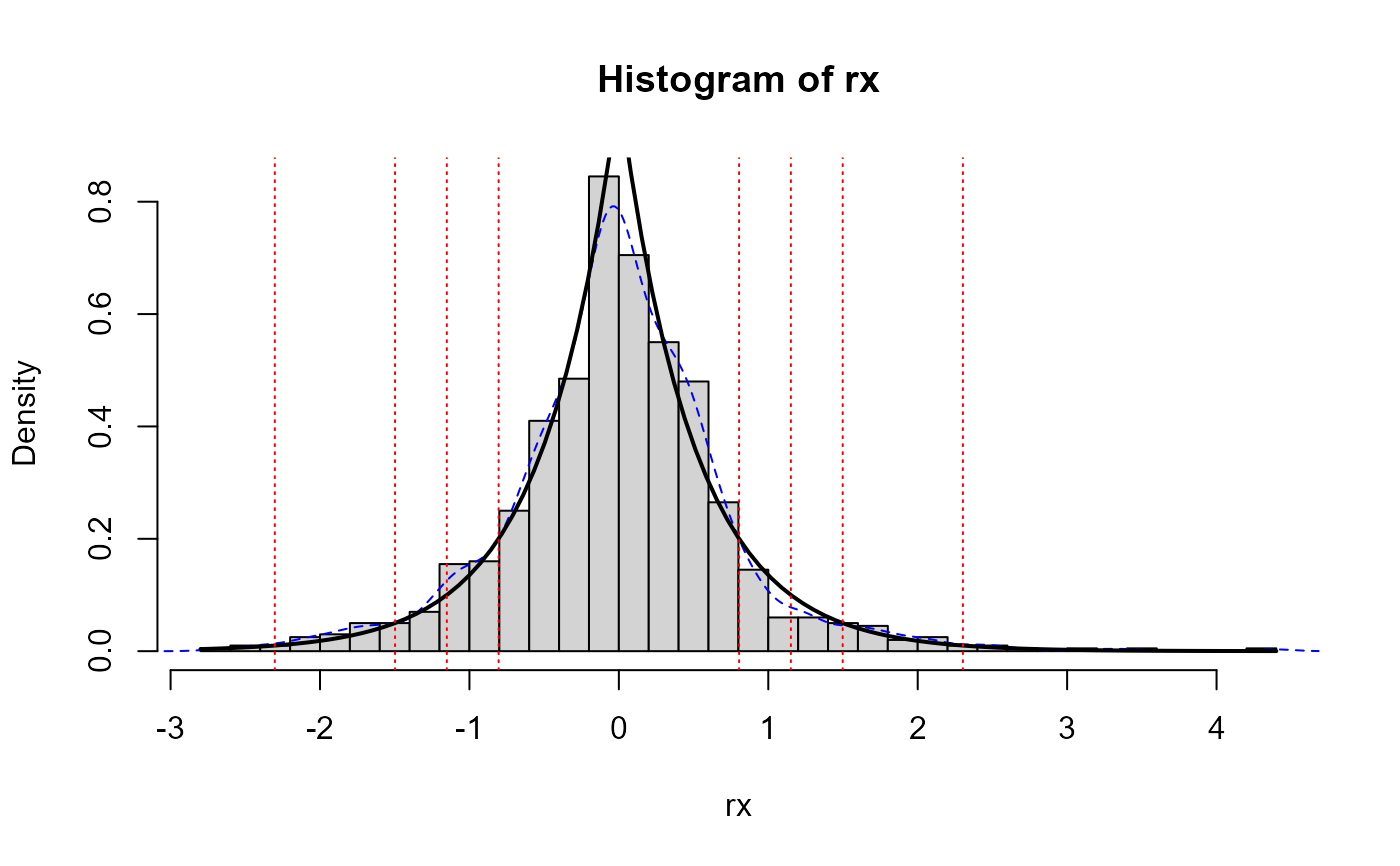
rx <- rdexp(10^3, rate)
hist(rx, breaks = "FD", freq = FALSE)
lines(density(rx), lty = 2, col = "blue")
curve(ddexp(x, rate), lwd = 2, add = TRUE)
p <- c(0.005, 0.025, 0.05, 0.1)
abline(v = qdexp(c(p, 1-p), rate = rate), lty = 3, col = "red")
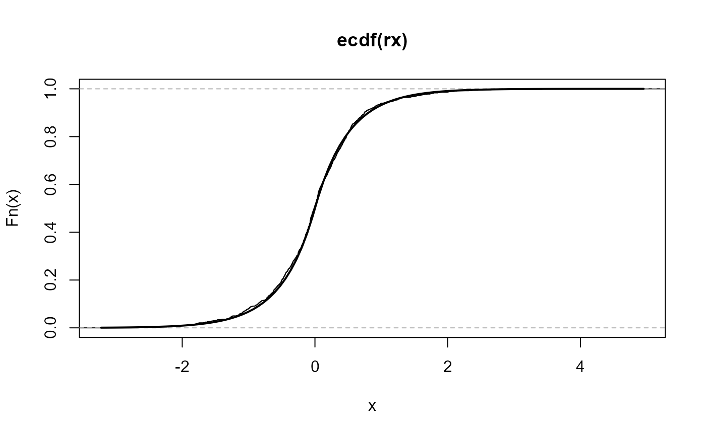
 plot(ecdf(rx))
curve(pdexp(x, rate), lwd = 2, add = TRUE)
plot(ecdf(rx))
curve(pdexp(x, rate), lwd = 2, add = TRUE)