Exploratory plots of a random sequence

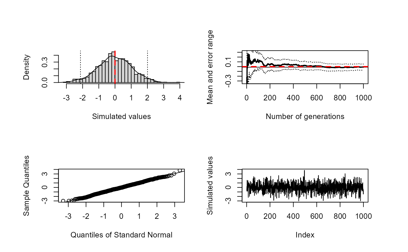
mc.plot() draws the approximation of the distribution, the convergence plot (by calling conv.plot()), a normal QQ plot and a sequential plot.

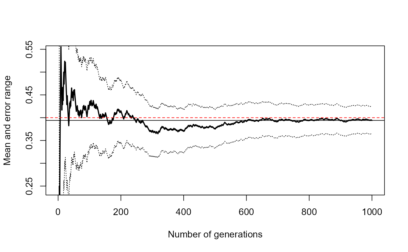
conv.plot() draws a convergence plot.

mc.integral() integrates an one-dimensional function over a bounded interval using classic Monte-Carlo integration and draws the corresponding convergence plot.

mc.plot(
  x,
  level = 0.95,
  true.value = NULL,
  main,
  omd = c(0.05, 0.95, 0.01, 0.95),
  ...
)

conv.plot(
  x,
  level = 0.95,
  lty = c(conv = 1, value = 1, error = 3),
  lwd = c(conv = 2, value = 1, error = 1),
  ylim = NULL,
  xlab = "Number of generations",
  ylab = "Mean and error range",
  ...
)

mc.integral(fun, a, b, n, level = 0.95, plot = TRUE, ...)

Arguments

x

the simulated values.

level

the confidence level required.

true.value

the theoretical value.

main

an overall title for the plot.

omd

a vector of the form c(x1, x2, y1, y2) giving the region inside outer margins in normalized device coordinates (i.e. fractions of the device region).

...

further arguments passed to other functions (e.g. to conv.plot()).

lty

a vector of line types (of the form c(conv, value, error)).

lwd

a vector of line widths (of the form c(conv, value, error)).

ylim

the y limits of the plot.

xlab, ylab

the axis titles.

fun

an one-dimensional function to be integrated on [a, b]

a, b

the limits of integration (must be finite).

n

number of uniform generations.

plot

logical; if TRUE a convergence plot is draw.

Value

Return, invisibly in the case of plot functions, the approximation by simulation (the arithmetic mean) and the corresponding error range (half width of the confidence interval).

Examples

set.seed(1)
teor <- 0
res <- mc.plot(rnorm(1000, mean = teor), true.value = teor)

res
#> $approx
#> [1] -0.01164814
#> 
#> $max.error
#> [1] 0.06414357
#> 
set.seed(1)
p <- 0.4
res <- conv.plot(rbinom(1000, size = 1, prob = p))
abline(h = p, lty = 2, col = "red") # Theoretical value

res
#> $approx
#> [1] 0.394
#> 
#> $max.error
#> [1] 0.0303005
#> 
fun <- function(x) ifelse((x > 0) & (x < 1), 4 * x^4, 0)
curve(fun, 0, 1)
abline(h = 0, lty = 2)
abline(v = c(0, 1), lty = 2)

set.seed(1)
mc.integral(fun, 0, 1, 1000)
#> $approx
#> [1] 0.8048108
#> 
#> $max.error
#> [1] 0.06752324
#> 
abline(h = 4/5, lty = 2, col = "red") # Theoretical value

set.seed(1)
mc.integral(fun, 0, 1, 5000, plot = FALSE)
#> $approx
#> [1] 0.8142206
#> 
#> $max.error
#> [1] 0.03028194
#>