splot() is designed to combine a standard R plot with
a legend representing a (continuous) color scale. This is done by splitting
the plotting region into two parts. Keeping one for the main chart and
putting the legend in the other.
Usage
splot(
  slim = c(0, 1),
  col = jet.colors(128),
  breaks = NULL,
  horizontal = FALSE,
  legend.shrink = 0.9,
  legend.width = 1.2,
  legend.mar = ifelse(horizontal, 3.1, 5.1),
  legend.lab = NULL,
  bigplot = NULL,
  smallplot = NULL,
  lab.breaks = NULL,
  axis.args = NULL,
  legend.args = NULL,
  add = FALSE
)
Arguments
- slim
limits used to set up the color scale.
- col
color table used to set up the color scale (see
imagefor details).- breaks
(optional) numeric vector with the breakpoints for the color scale: must have one more breakpoint than
coland be in increasing order.- horizontal
logical; if
FALSE(default) legend will appear on the right side. IfTRUEthe legend will be along the bottom.- legend.shrink
amount to shrink the size of legend relative to the full height or width of the plot.
- legend.width
width in characters of the legend strip. Default is 1.2, a little bigger that the width of a character.
- legend.mar
width in characters of legend margin that has the axis. Default is 5.1 for a vertical legend and 3.1 for a horizontal legend.
- legend.lab
label for the axis of the color legend. Default is no label as this is usual evident from the plot title.
- bigplot
plot coordinates for main plot. If not passed these will be determined within the function.
- smallplot
plot coordinates for legend strip. If not passed these will be determined within the function.
- lab.breaks
if breaks are supplied these are text string labels to put at each break value. This is intended to label axis on a transformed scale such as logs.
- axis.args
additional arguments for the axis function used to create the legend axis (see
image.plotfor details).- legend.args
arguments for a complete specification of the legend label. This is in the form of list and is just passed to the
mtextfunction. Usually this will not be needed (seeimage.plotfor details).- add
logical; if
TRUEthe legend is just added to the existing plot (the graphical parameters are not changed).
Value
Invisibly returns a list with the following 3 components:
- bigplot
plot coordinates of the main plot. These values may be useful for drawing a plot without the legend that is the same size as the plots with legends.
- smallplot
plot coordinates of the secondary plot (legend strip).
- old.par
previous graphical parameters (
par(old.par)will reset plot parameters to the values before entering the function).
Details
For instance, sxxxx() functions (spoints(), simage()
and spersp()) draw the corresponding high-level plot (xxxx()),
after calling splot(), to include a legend strip for the color scale.
These functions are based on function image.plot of package
fields, see its documentation for additional information.
Side Effects
The plotting region (par("plt")) may be changed
after exiting, to make it possible to add more features to the plot.
They can be restored using the old.par returned values or by calling
function par.reset().
See also
jet.colors, hot.colors, scolor,
spoints, simage, spersp,
image, image.plot.
Author
Based on image.plot function from package fields:
fields, Tools for spatial data.
Copyright 2004-2013, Institute for Mathematics Applied Geosciences.
University Corporation for Atmospheric Research.
Modified by Ruben Fernandez-Casal rubenfcasal@gmail.com.
Examples
# Plot equivalent to spoints():
scale.range <- range(mtcars$mpg)
res <- splot(slim = scale.range, legend.lab = "mpg")
with(mtcars,
plot(hp, qsec, col = scolor(mpg, slim = scale.range),
pch = 16, cex = 1.5, main = "Motor Trend Car Road Tests")
)
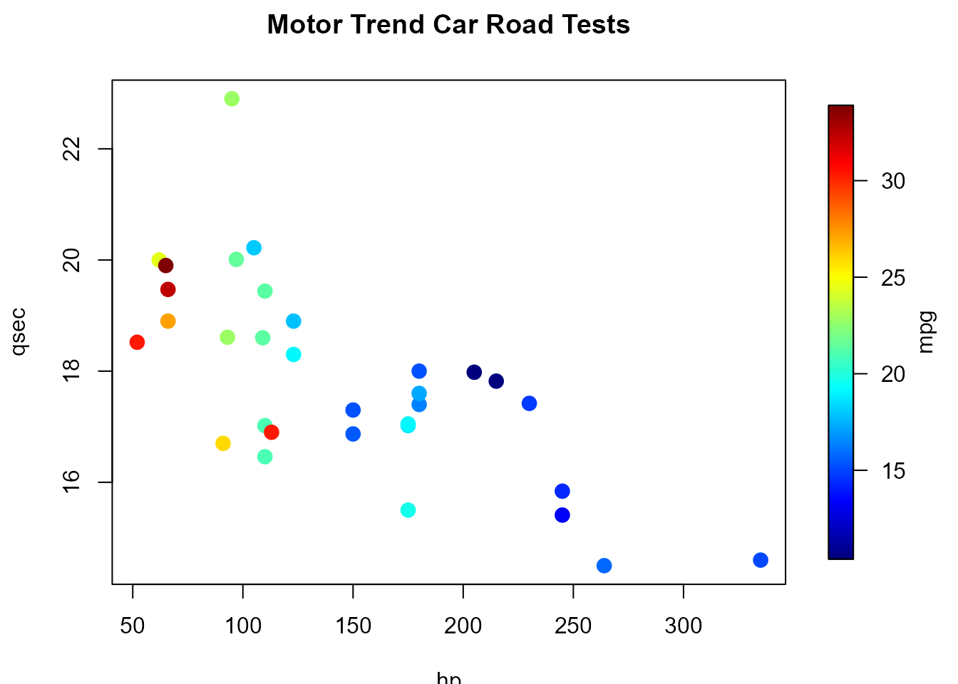 par(res$old.par) # restore graphical parameters
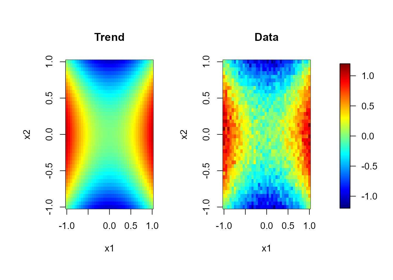
# Multiple plots with a common legend:
# regularly spaced 2D data...
set.seed(1)
nx <- c(40, 40) # ndata = prod(nx)
x1 <- seq(-1, 1, length.out = nx[1])
x2 <- seq(-1, 1, length.out = nx[2])
trend <- outer(x1, x2, function(x,y) x^2 - y^2)
y <- trend + rnorm(prod(nx), 0, 0.1)
scale.range <- c(-1.2, 1.2)
scale.color <- jet.colors(256)
# 1x2 plot with some room for the legend...
old.par <- par(mfrow = c(1,2), omd = c(0.05, 0.85, 0.05, 0.95))
image( x1, x2, trend, zlim = scale.range, main = 'Trend', col = scale.color)
image( x1, x2, y, zlim = scale.range, main = 'Data', col = scale.color)
par(old.par)
# the legend can be added to any plot...
splot(slim = scale.range, col = scale.color, legend.shrink = 0.7, add = TRUE)
par(res$old.par) # restore graphical parameters
# Multiple plots with a common legend:
# regularly spaced 2D data...
set.seed(1)
nx <- c(40, 40) # ndata = prod(nx)
x1 <- seq(-1, 1, length.out = nx[1])
x2 <- seq(-1, 1, length.out = nx[2])
trend <- outer(x1, x2, function(x,y) x^2 - y^2)
y <- trend + rnorm(prod(nx), 0, 0.1)
scale.range <- c(-1.2, 1.2)
scale.color <- jet.colors(256)
# 1x2 plot with some room for the legend...
old.par <- par(mfrow = c(1,2), omd = c(0.05, 0.85, 0.05, 0.95))
image( x1, x2, trend, zlim = scale.range, main = 'Trend', col = scale.color)
image( x1, x2, y, zlim = scale.range, main = 'Data', col = scale.color)
par(old.par)
# the legend can be added to any plot...
splot(slim = scale.range, col = scale.color, legend.shrink = 0.7, add = TRUE)
 ## note that argument 'zlim' in 'image' corresponds with 'slim' in 'sxxxx' functions.