Introduction to the scimetr package

library(scimetr)

##  scimetr: Analysis of Scientific Publication Data with R,
##  version 1.1.0 (built on 2025-11-22).
##  Copyright (C) UDC Rankings Group 2017-2025.
##  Type `help(scimetr)` for an overview of the package or
##  visit https://rubenfcasal.github.io/scimetr.

This vignette illustrates the use of the scimetr package for performing bibliometric analyses using datasets exported from Web of Science, highlighting the main workflows and functionalities. The package provides tools for scientometric and bibliometric research, including routines to import bibliographic records from Clarivate Analytics Web of Science (WoS) and conduct bibliometric analyses.

A list of other useful R packages for this type of analysis is available here.

Installation

Since the package is not yet available on CRAN, you need to install the development version from the GitHub repository rubenfcasal/scimetr:

# install.packages("remotes")
remotes::install_github("rubenfcasal/mpae")

Alternatively, Windows users may install the corresponding scimetr_X.Y.Z.zip file in the releases section of the github repository. It is recommended to first install its dependencies:

# Dependencies
install.packages(c('dplyr', 'tidyr', 'stringr', 'ggplot2', 'scales', 'rlang'))
# Last released version
install.packages('https://github.com/rubenfcasal/scimetr/releases/download/v1.1.0/scimetr_1.1.0.zip', repos = NULL)

Once the package is installed, it can be loaded as usual.

Bibliographic data

We will focus exclusively on importing publication data from WoS in text format. First, you need to download the corresponding files from the WoS website, for example, by following the steps described here.

Loading WoS data from a directory

WoS files (which by default are limited to 500 records each) can be automatically loaded from a subdirectory:

dir("UDC_2018-2023 (01-02-2024)", pattern = "*.txt")

##  [1] "savedrecs01.txt" "savedrecs02.txt" "savedrecs03.txt" "savedrecs04.txt"
##  [5] "savedrecs05.txt" "savedrecs06.txt" "savedrecs07.txt" "savedrecs08.txt"
##  [9] "savedrecs09.txt" "savedrecs10.txt"

To combine the files into a data.frame, the ImportSources.wos() function is used:

wos.data <- ImportSources.wos("UDC_2018-2023 (01-02-2024)")

Next, the database must be created using the CreateDB() function, as shown later.

Example data

The package includes the example dataset wosdf (obtained using the ImportSources.wos() function), corresponding to a WoS search by the Affiliation field of Universidade da Coruña (UDC) (Affiliation: OG = Universidade da Coruna) in the research area "Mathematics" during the years 2018–2023.

All data tables have an associated variable.labels attribute with the variable labels. These will be displayed below the variable names when viewed in RStudio (e.g. View(wosdf)).

wos.labels <- attr(wosdf, "variable.labels")
knitr::kable(head(data.frame(wos.labels)),
             col.names = c("Variable", "Label"))

Variable	Label
PT	Publication Type
AU	Author
AF	Author Full Name
TI	Article Title
SO	Source Title
SE	Book Series Title

…

A full list of the variables used in the database tables is shown in the final section Variable list of this document.

Bibliographic database

scimetr uses lists with data.frame components as relational databases.

To create the bibliographic database, use the CreateDB() function (the result is a wos.db-class S3 object):

db <- CreateDB(wosdf, label = "Mathematics_UDC_2018-2023")
names(db)

##  [1] "Docs"         "Authors"      "AutDoc"       "OI"           "OIDoc"       
##  [6] "RI"           "RIDoc"        "Categories"   "CatSour"      "Areas"       
## [11] "AreaSour"     "Addresses"    "AddAutDoc"    "Affiliations" "AffDoc"      
## [16] "Sources"      "WSIndex"      "SourWSI"      "label"        "export.date"

Summaries

You can generate either global summaries or yearly summaries of your database.

Global summary

The summary() method of a bibliographic database (summary.wos.db()), provides an overview of the entire database, including total documents, authors, journals, citations, and other aggregated statistics.

res1 <- summary(db)
options(digits = 5)
res1

## Number of documents: 293 
## Authors: 504 
## Period: 2018 - 2023 
## 
## Document types:
##                            Documents
## Article                          254
## Article; Early Access              1
## Article; Proceedings Paper         2
## Correction                         7
## Editorial Material                21
## Review                             8
## 
## Number of authors per document:
##    Min. 1st Qu.  Median    Mean 3rd Qu.    Max. 
##    1.00    3.00    3.00    3.63    4.00   13.00 
## 
## Number of documents per author:
##    Min. 1st Qu.  Median    Mean 3rd Qu.    Max. 
##    1.00    1.00    1.00    2.11    2.00   23.00 
## 
## Number of times cited:
##    Min. 1st Qu.  Median    Mean 3rd Qu.    Max. 
##    0.00    1.00    3.00    5.87    7.00  123.00 
## 
## Indexes:
##  H  G 
## 19 27 
## 
## Status:
## Highly Cited   Hot Papers 
##            1            0 
## 
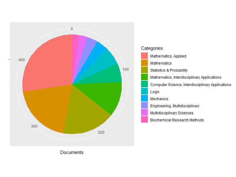
## Top Categories:
##                                                  Documents
## Mathematics, Applied                                   133
## Mathematics                                             96
## Statistics & Probability                                84
## Mathematics, Interdisciplinary Applications             55
## Computer Science, Interdisciplinary Applications        30
## Logic                                                   28
## Mechanics                                               19
## Engineering, Multidisciplinary                          17
## Multidisciplinary Sciences                              13
## Biochemical Research Methods                            11
## Others                                                 104
## 
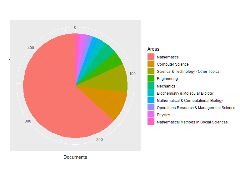
## Top Areas:
##                                          Documents
## Mathematics                                    293
## Computer Science                                45
## Science & Technology - Other Topics             41
## Engineering                                     20
## Mechanics                                       19
## Biochemistry & Molecular Biology                11
## Mathematical & Computational Biology             9
## Operations Research & Management Science         9
## Physics                                          9
## Mathematical Methods In Social Sciences          7
## Others                                          37
## 
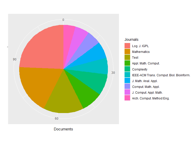
## Top Journals:
##                                          Documents
## Log. J. IGPL                                    28
## Mathematics                                     21
## Test                                            17
## Appl. Math. Comput.                              9
## Complexity                                       9
## IEEE-ACM Trans. Comput. Biol. Bioinform.         7
## J. Math. Anal. Appl.                             7
## Comput. Math. Appl.                              6
## J. Comput. Appl. Math.                           6
## Arch. Comput. Method Eng.                        5
## Others                                         178
## 
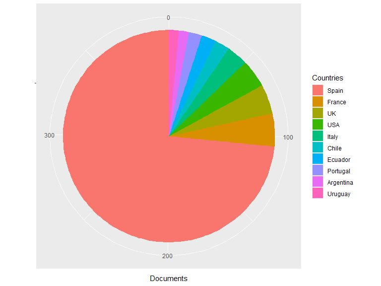
## Top Countries:
##           Documents
## Spain           293
## France           20
## UK               18
## USA              17
## Italy            13
## Chile             9
## Ecuador           9
## Portugal          8
## Argentina         6
## Uruguay           6
## Others           46
## 
## International colaboration documents (Spain): 134

Yearly summary

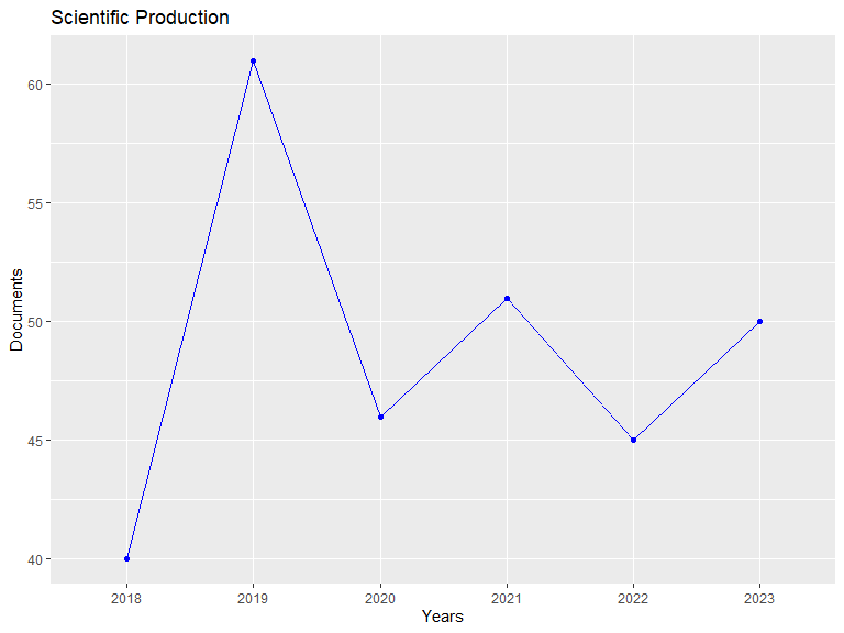
The summary_year() method breaks down the summary by year, showing trends over time in publications, citations, and other key metrics.

res2 <- summary_year(db)
res2

## Annual Scientific Production:
##      Documents
## 2018        40
## 2019        61
## 2020        46
## 2021        51
## 2022        45
## 2023        50
## 
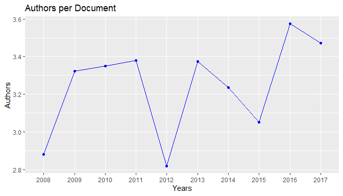
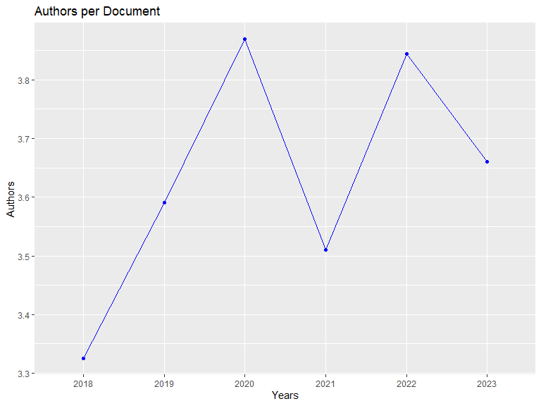
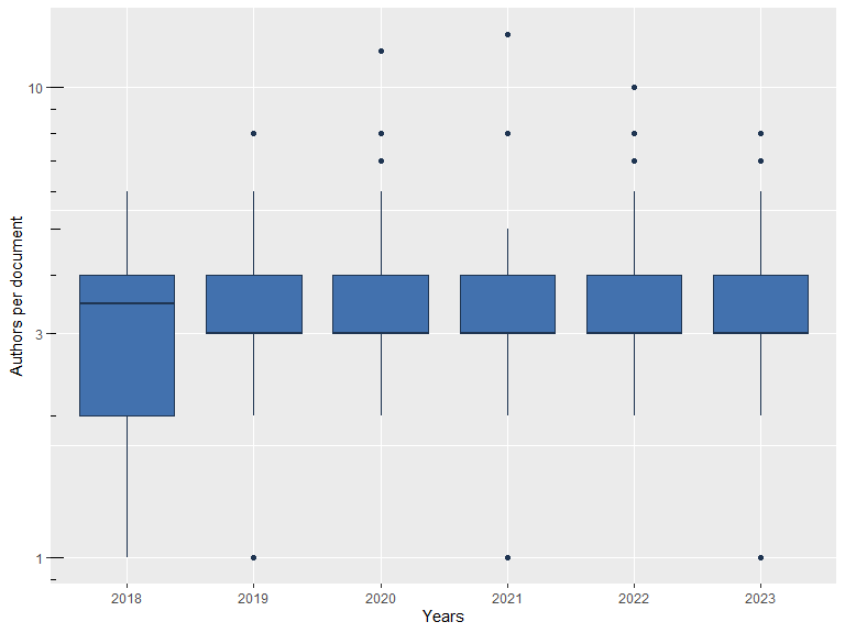
## Annual Authors per Document:
##    PY   Mean Median
##  2018 3.3250    3.5
##  2019 3.5902    3.0
##  2020 3.8696    3.0
##  2021 3.5098    3.0
##  2022 3.8444    3.0
##  2023 3.6600    3.0
## 
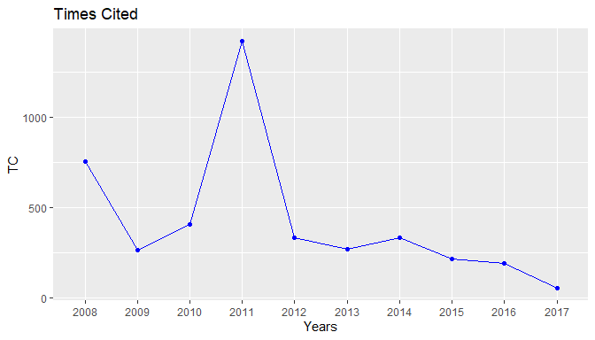
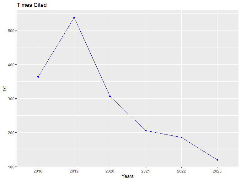
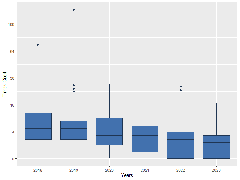
## Annual Times Cited:
##    PY Cites   Mean Median
##  2018   364 9.1000    5.0
##  2019   538 8.8197    5.0
##  2020   306 6.6522    3.0
##  2021   206 4.0392    3.0
##  2022   186 4.1333    2.0
##  2023   120 2.4000    1.5
## 
## Status:
##    PY Highly Cited Hot Paper
##  2018            0         0
##  2019            1         0
##  2020            0         0
##  2021            0         0
##  2022            0         0
##  2023            0         0

Visualizations

The ggplot2 package is used to create a wide variety of visualizations from the database.
There are three main types of plots you can create:

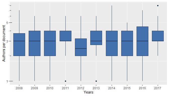
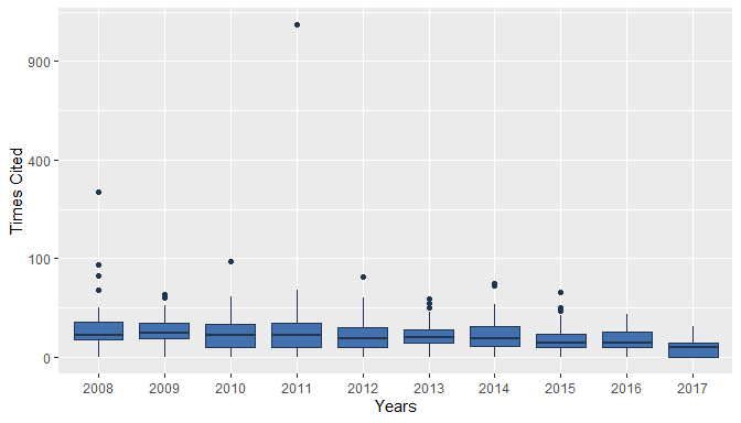
Database plots (plot(db)).
Summary plots (plot(summary(db)).
Yearly summary plots (plot(summary_year(db))).

Note: All plot() methods invisible return a list with the generated ggplot2 objects (use plot = FALSE to avoid plotting).

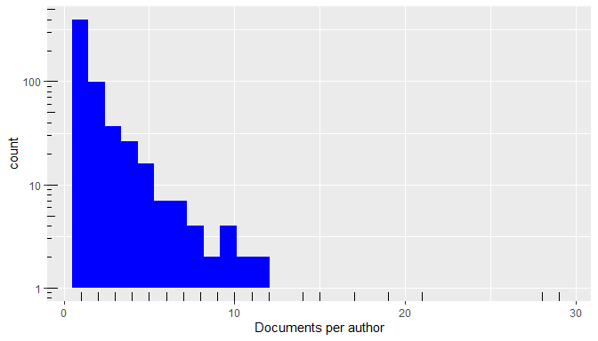
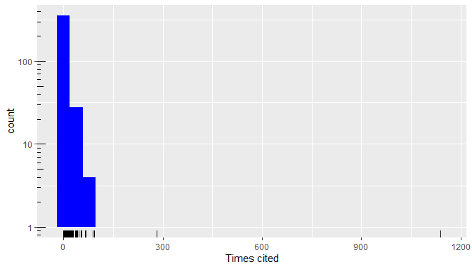
Database plots

The plot() method of a bibliographic database (plot.wos.db()) provides a general visualization of its contents.

plot(db)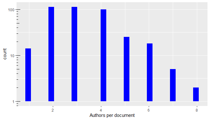

Summary plots

The plot method of a summary result (plot.summary.wos.db()) visualizes the results generating different types of plots: standard bar, line plots or Pie charts (pie = TRUE).

plot(res1)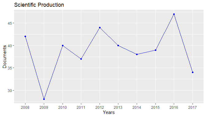

plot(res1, pie = TRUE)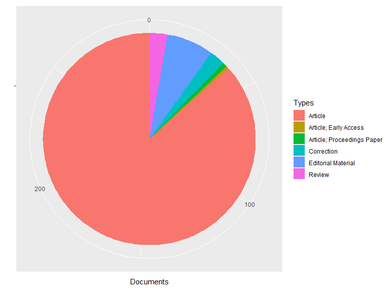

Yearly summary plots

The plot() method of a yearly summary (plot.summary.year()) visualizes the results generating different types of plots: standard bar and line plots for trends over time, or boxplots (boxplot = TRUE), to show variability within each year.

plot(res2)

plot(res2, boxplot = TRUE)

Filtering

To filter elements (entities) of the database, you can use the functions get.id<Table>() to retrieve identification codes (IDs or entity key values). Any variable from the corresponding <Table> may be used (multiple conditions are combined with &; see e.g. dplyr::filter()).

Typically, these functions are combined together with the get.idDocs() function to obtain document IDs, which are finally used in argument filter of summary functions to filter documents in results.

Retrieving element IDs (entity key values)

get.idAuthors(): Retrieve author IDs (codes)

Search for a specific author:

idAuthor <- get.idAuthors(db, AF == "Cao, Ricardo")
idAuthor

## Cao, Ricardo Cao, Ricardo 
##           11          260

Search by partial name match:

idAuthors <- get.idAuthors(db, grepl('Cao', AF))
idAuthors

##      Cao, Ricardo   Cao-Rial, M. T.      Cao, Ricardo           Cao, R. 
##                11                80               260               328 
## Cao Abad, Ricardo   Cao-Rial, M. T. 
##               501               504

get.idAreas(): Retrieve codes for research areas

get.idAreas(db, SC == 'Mathematics')

## Mathematics 
##          16

get.idAreas(db, SC == 'Mathematics' | SC == 'Computer Science')

## Computer Science      Mathematics 
##                6               16

get.idCategories(): Retrieve category codes

get.idCategories(db, grepl('Mathematics', WC))

##                                 Mathematics 
##                                         148 
##                        Mathematics, Applied 
##                                         149 
## Mathematics, Interdisciplinary Applications 
##                                         150

get.idSources(): Retrieve source codes (journals, books, or collections)

ijss <- get.idSources(db, SO == 'TEST')
ijss

## TEST 
##    6

knitr::kable(t(db$Sources[ijss, ]), caption = "Test journal",
             col.names = c("Variable", "Value"))

Test journal
Variable	Value
ids	6
PT	Journal
SO	TEST
SE	NA
BS	NA
LA	English
PU	SPRINGER
PI	NEW YORK
PA	ONE NEW YORK PLAZA, SUITE 4600, NEW YORK, NY, UNITED STATES
SN	1133-0686
EI	1863-8260
BN	NA
J9	TEST-SPAIN
JI	Test

# get.idSources(db, JI == 'Test')

Retrieving documents IDs (by authors, journals, etc.)

The IDs retrieved above can be combined in get.idDocs():

idocs <- get.idDocs(db, idAuthors = idAuthor)
idocs

##  [1]   6  14  66  94 102 104 148 162 164 170 171 187 225 286 287 288

The document IDs can be used as filters, for example, in summary.wos.db().

Filtered Summaries

Get a summary for one or more authors:

summary(db, idocs)

## Number of documents: 16 
## Authors: 21 
## Period: 2019 - 2023 
## 
## Document types:
##                    Documents
## Article                   10
## Editorial Material         5
## Review                     1
## 
## Number of authors per document:
##    Min. 1st Qu.  Median    Mean 3rd Qu.    Max. 
##    1.00    2.00    3.00    2.81    3.25    5.00 
## 
## Number of documents per author:
##    Min. 1st Qu.  Median    Mean 3rd Qu.    Max. 
##    1.00    1.00    1.00    2.14    2.00    9.00 
## 
## Number of times cited:
##    Min. 1st Qu.  Median    Mean 3rd Qu.    Max. 
##    0.00    0.00    2.50   11.81    6.75  123.00 
## 
## Indexes:
##  H  G 
##  5 13 
## 
## Status:
## Highly Cited   Hot Papers 
##            1            0 
## 
## Top Categories:
##                                                  Documents
## Statistics & Probability                                15
## Operations Research & Management Science                 2
## Computer Science, Interdisciplinary Applications         1
## Mathematical & Computational Biology                     1
## Mathematics                                              1
## Medical Informatics                                      1
## Medicine, Research & Experimental                        1
## Public, Environmental & Occupational Health              1
## 
## Top Areas:
##                                             Documents
## Mathematics                                        16
## Operations Research & Management Science            2
## Computer Science                                    1
## Mathematical & Computational Biology                1
## Medical Informatics                                 1
## Public, Environmental & Occupational Health         1
## Research & Experimental Medicine                    1
## 
## Top Journals:
##                                       Documents
## Test                                          4
## J. Nonparametr. Stat.                         2
## J. Multivar. Anal.                            2
## SORT-Stat. Oper. Res. Trans.                  2
## Mathematics                                   1
## Comput. Stat.                                 1
## Commun. Stat.-Simul. Comput.                  1
## Stat. Med.                                    1
## J. Stat. Comput. Simul.                       1
## Wiley Interdiscip. Rev.-Comput. Stat.         1
## 
## Top Countries:
##             Documents
## Spain              16
## France              3
## Uruguay             2
## Belgium             1
## Canada              1
## Mexico              1
## Switzerland         1
## USA                 1
## 
## International colaboration documents (Spain): 7

Get a year-by-year summary for one or more authors:

summary_year(db, idocs)

## Annual Scientific Production:
##      Documents
## 2019         6
## 2020         2
## 2021         3
## 2022         3
## 2023         2
## 
## Annual Authors per Document:
##    PY   Mean Median
##  2019 3.1667    3.5
##  2020 3.0000    3.0
##  2021 2.6667    3.0
##  2022 2.6667    3.0
##  2023 2.0000    2.0
## 
## Annual Times Cited:
##    PY Cites   Mean Median
##  2019   166 27.667   10.5
##  2020    11  5.500    5.5
##  2021     6  2.000    0.0
##  2022     6  2.000    2.0
##  2023     0  0.000    0.0
## 
## Status:
##    PY Highly Cited Hot Paper
##  2019            1         0
##  2020            0         0
##  2021            0         0
##  2022            0         0
##  2023            0         0

Author metrics

Retrieve metrics for multiple authors:

TC.authors(db, idAuthors)

##                   H G
## Cao, Ricardo      3 9
## Cao-Rial, M. T.   4 5
## Cao, Ricardo      4 5
## Cao, R.           0 0
## Cao Abad, Ricardo 1 2
## Cao-Rial, M. T.   0 0

Bibliographic database with JCR metrics

We can extends the bibliographic database by adding JCR metrics to sources, per year and WoS category.

Import JCR data from WoS

Excel files with JCR data (avaliable from WoS) can be automatically loaded from a subdirectory:

dir("JCR_download", pattern = "*.xlsx")

##  [1] "JCR_SCIE_2018.xlsx" "JCR_SCIE_2019.xlsx" "JCR_SCIE_2020.xlsx"
##  [4] "JCR_SCIE_2021.xlsx" "JCR_SCIE_2022.xlsx" "JCR_SCIE_2023.xlsx"
##  [7] "JCR_SSCI_2018.xlsx" "JCR_SSCI_2019.xlsx" "JCR_SSCI_2020.xlsx"
## [10] "JCR_SSCI_2021.xlsx" "JCR_SSCI_2022.xlsx" "JCR_SSCI_2023.xlsx"

To combine the files into a relational database, the CreateDBJCR() function is used:

jcr <- CreateDBJCR("JCR_download")

Add JCR data to a bibliographic database

The JCR data can be combined with a bibliographic database by using the AddDBJCR() function:

dbjcr <- AddDBJCR(db, jcr)

Two additional tables, JCRSour and JCRCatSour, are added to the bibliographic database (the result is a wos.jcr-class S3 object).

The database resulting from this particular example is provided as a dataset of the scimetr package:

names(dbjcr)

##  [1] "Docs"         "Authors"      "AutDoc"       "OI"           "OIDoc"       
##  [6] "RI"           "RIDoc"        "Categories"   "CatSour"      "Areas"       
## [11] "AreaSour"     "Addresses"    "AddAutDoc"    "Affiliations" "AffDoc"      
## [16] "Sources"      "WSIndex"      "SourWSI"      "label"        "export.date" 
## [21] "JCRSour"      "JCRCatSour"

class(dbjcr)

## [1] "wos.jcr" "wos.db"

Summaries

Auxiliary functions are available to perform database queries:

get_jcr(): combines document indexes with their source JCR metrics per year.

head(get_jcr(dbjcr))

##   idd ids   PY   JIF   IMM  CHL   JIF5     JEF     JEFN   JAI
## 1   1   1 2021 1.673 0.165  4.9 11.808 0.01332  2.86423 4.500
## 2   2   2 2018 2.896 1.169  4.7  2.344 0.00585  0.69599 0.707
## 3   3   3 2023 2.300 0.900  1.9  2.200 0.03686  8.10075 0.374
## 4   4   4 2023 4.400 1.000  3.2  3.600 0.00847  1.86316 0.691
## 5   5   5 2023 4.400 1.000 10.0  7.600 0.12386 27.21696 3.056
## 6   6   6 2023 1.200 0.200  7.7  2.200 0.00235  0.51687 1.225

get_jcr_cat() combines document indexes with their source JCR metrics per year and WoS category (if best = TRUE, only the results for the WoS category with the best ranking for each document are returned).

head(get_jcr_cat(dbjcr, best = TRUE))

##   idd ids   PY idc     WCR JIFQ   JIFP   WE WCP WCT
## 1   1   1 2021  46 0.13514   Q4 13.840 SCIE  97 112
## 2   2   2 2018  46 0.65714   Q2 65.566 SCIE  37 106
## 3   3   3 2023 148 0.95910   Q1 95.800 SCIE  21 490
## 4   4   4 2023  46 0.78107   Q1 77.900 SCIE  38 170
## 5   5   5 2023  26 0.78613   Q1 78.400 SCIE  38 174
## 6   6   6 2023 237 0.56287   Q2 56.300 SCIE  74 168

The summary methods combine the above queries and generate global summaries or yearly summaries of a bibliographic database with JCR metrics (if all = TRUE, the corresponding wos.db-class results are also generated).

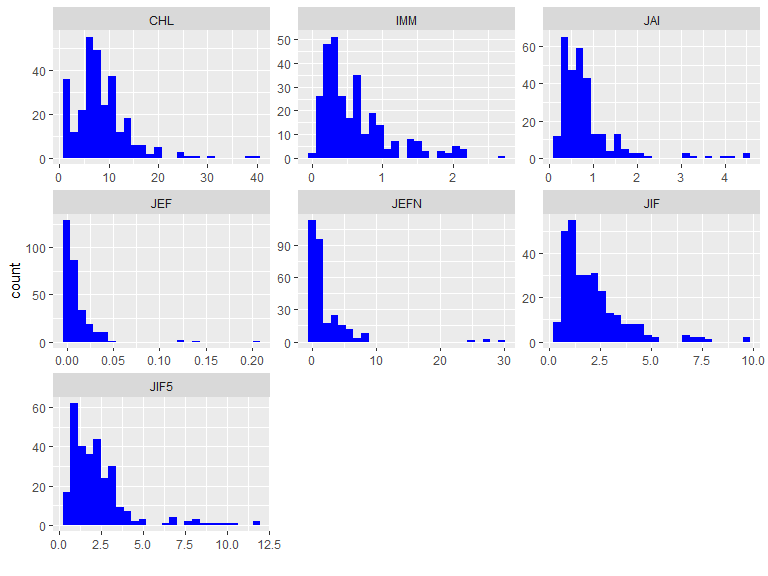
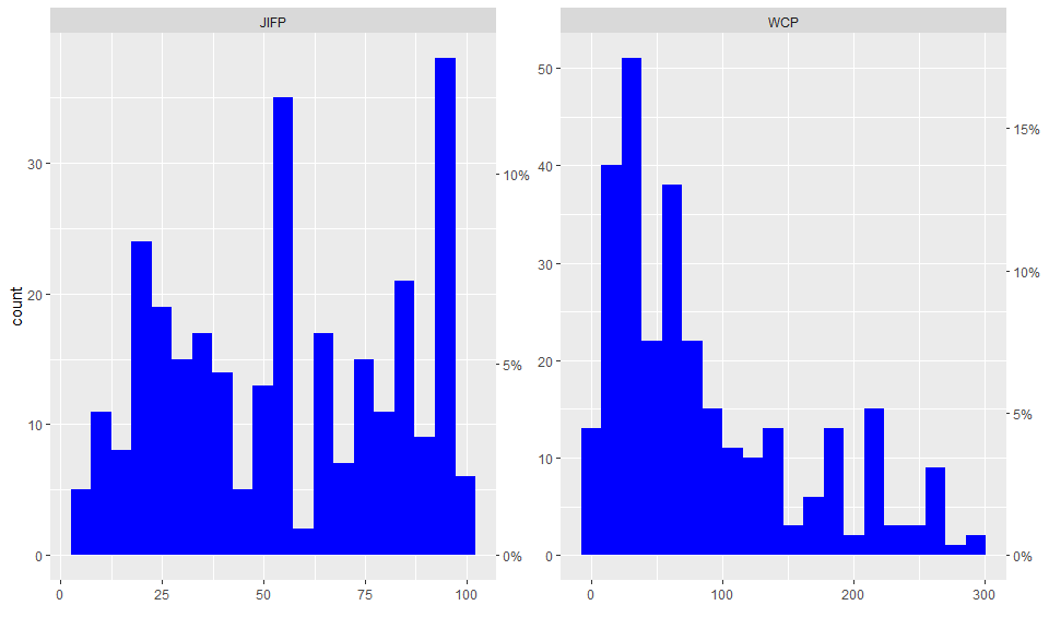
res1 <- summary(dbjcr)
res1

## JCR metrics:
##         JIF  IMM  CHL  JIF5     JEF   JEFN  JAI JIFP WCP
## Min.    0.4 0.00  1.1  0.48 0.00042  0.053 0.18  2.8   5
## 1st Qu. 1.0 0.26  5.6  1.00 0.00226  0.381 0.42 28.6  31
## Median  1.7 0.45  7.7  1.87 0.00500  0.848 0.66 56.3  58
## Mean    2.1 0.62  8.6  2.30 0.01119  2.060 0.83 55.1  86
## 3rd Qu. 2.6 0.83 10.4  2.73 0.01412  2.352 0.89 82.6 126
## Max.    9.7 2.69 39.5 11.81 0.20530 29.627 4.50 97.6 298
## NA's    1.0 1.00  1.0  2.00 1.00000  1.000 2.00  1.0   1
## 
## Documents in JCR: 292 (99.66%)
## Documents in Q1: 90 (30.82% of JCR)
## Documents in D1: 50 (17.12% of JCR)
## Documents in top 3 journals: 0 (0% of JCR)

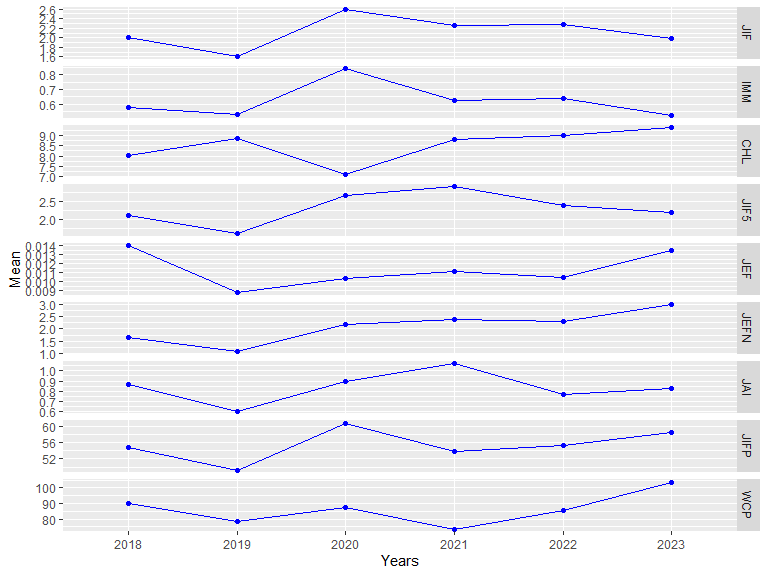
res2 <- summary_year(dbjcr)
res2

## Mean of JCR metrics:
##    PY  JIF   IMM  CHL JIF5     JEF JEFN   JAI JIFP   WCP
##  2018 2.01 0.579 8.03 2.11 0.01397 1.66 0.864 54.8  89.7
##  2019 1.60 0.527 8.85 1.61 0.00876 1.07 0.605 49.3  78.4
##  2020 2.59 0.841 7.09 2.68 0.01030 2.16 0.899 60.8  87.2
##  2021 2.27 0.624 8.81 2.92 0.01108 2.38 1.068 53.7  73.5
##  2022 2.28 0.638 8.98 2.39 0.01050 2.29 0.769 55.3  85.2
##  2023 1.98 0.520 9.38 2.21 0.01349 2.97 0.830 58.4 103.7
## 
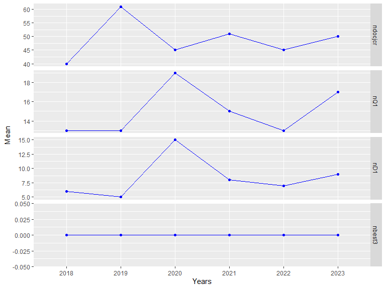
## Documents in JCR:
## 2018 2019 2020 2021 2022 2023 
##   40   61   45   51   45   50 
## 
## Documents in Q1:
## 2018 2019 2020 2021 2022 2023 
##   13   13   19   15   13   17 
## 
## Documents in D1:
## 2018 2019 2020 2021 2022 2023 
##    6    5   15    8    7    9 
## 
## Documents in top 3 journals:
## 2018 2019 2020 2021 2022 2023 
##    0    0    0    0    0    0

Note: res1$docjcrcat contains the combined queries.

Visualizations

The plot() method (plot.wos.jcr()) generates histograms of documents JCR metrics (if argument all = TRUE, plot.wos.bd() is also called):

plot(dbjcr)

Summary results have also a plot() method:

plot(res1)

plot(res2)

Variable list

The following list shows all variables used in the database tables:

Note: The table above was generated using the datatable() function from the DT package. By default, the first rows are displayed. Click on the page index (below) to change this. You can sort by column by clicking on the arrows to the right of its name. You can search for values (search box, top right) and filter values (click on the filter box below the name of each variable).

UDC Ranking’s Group

scimetr 1.1.0: 2025-11-22

Installation

Bibliographic data

Loading WoS data from a directory

Example data

Bibliographic database

Summaries

Global summary

Yearly summary

Visualizations

Database plots

Summary plots

Yearly summary plots

Filtering

Retrieving element IDs (entity key values)

Retrieving documents IDs (by authors, journals, etc.)

Filtered Summaries

Author metrics

Bibliographic database with JCR metrics

Import JCR data from WoS

Add JCR data to a bibliographic database

Summaries

Visualizations

Variable list