Local polynomial trend estimation

Estimates the functional mean (and its first derivatives) using local polynomial kernel smoothing.

# S3 method for npf.data
locpol(
  x,
  h = NULL,
  degree = 1 + as.numeric(drv),
  drv = FALSE,
  hat.bin = FALSE,
  ncv = 0,
  ...
)

# S3 method for npf.bin
locpol(
  x,
  h = NULL,
  degree = 1 + as.numeric(drv),
  drv = FALSE,
  hat.bin = FALSE,
  ncv = 0,
  ...
)

# S3 method for npf.locpol
predict(object, newx = NULL, ...)

# S3 method for npf.locpol
residuals(object, var, as.npf.data = TRUE, ...)

# S3 method for npf.locpol
plot(
  x,
  y = NULL,
  main = deparse(substitute(x)),
  col = "lightgray",
  legend = FALSE,
  ...
)

Arguments

x

an object (of class npf.data or npf.bin) used to select a method.

h

(full) bandwidth matrix (controls the degree of smoothing; only the upper triangular part of h is used).

degree

degree of the local polynomial used. Defaults to 1 (local linear estimation).

drv

logical; if TRUE, the matrix of estimated first derivatives is returned.

hat.bin

logical; if TRUE, the hat matrix of the binned data is returned.

ncv

integer; determines the number of cells leaved out in each dimension. Defaults to 0 (the full data is used) and it is not normally changed by the user in this setting. See "Details" below.

...

additional graphical parameters (passed to plot.npf.data).

object

object used to select a method.

newx

vector with the (irregular) points to predict (interpolate).

var

(optional) a vector or an object of class npf.var with the estimated (or theoretical) variances.

as.npf.data

logical; if TRUE (default) returns a npf.data-class object containing the residuals.

y

(optional) a vector or an object of class npf.var with the estimated (or theoretical) variances.

main

plot title.

col

color table used to set up the color scale (see image for details).

legend

logical; if TRUE (default), the plotting region is splitted into two parts, drawing the main plot in one and the legend with the color scale in the other. If FALSE only the (coloured) main plot is drawn and the arguments related to the legend are ignored (npsp::splot() is not called).

Value

locpol.npf.data and locpol.npf.bin return an S3 object of class npf.locpol extending npsp::locpol.bin (locpol + bin data + grid par.).

If newx == NULL, predict.npf.locpol returns the trend estimates corresponding to the discretization points (otherwise npsp::interp.data.grid is called).

residuals.npf.locpol returns the residuals, standardized if var

is not missing, and as a npf.data-class object if as.npf.data = TRUE.

See also

npsp::locpol.bin, npf.bin

Examples

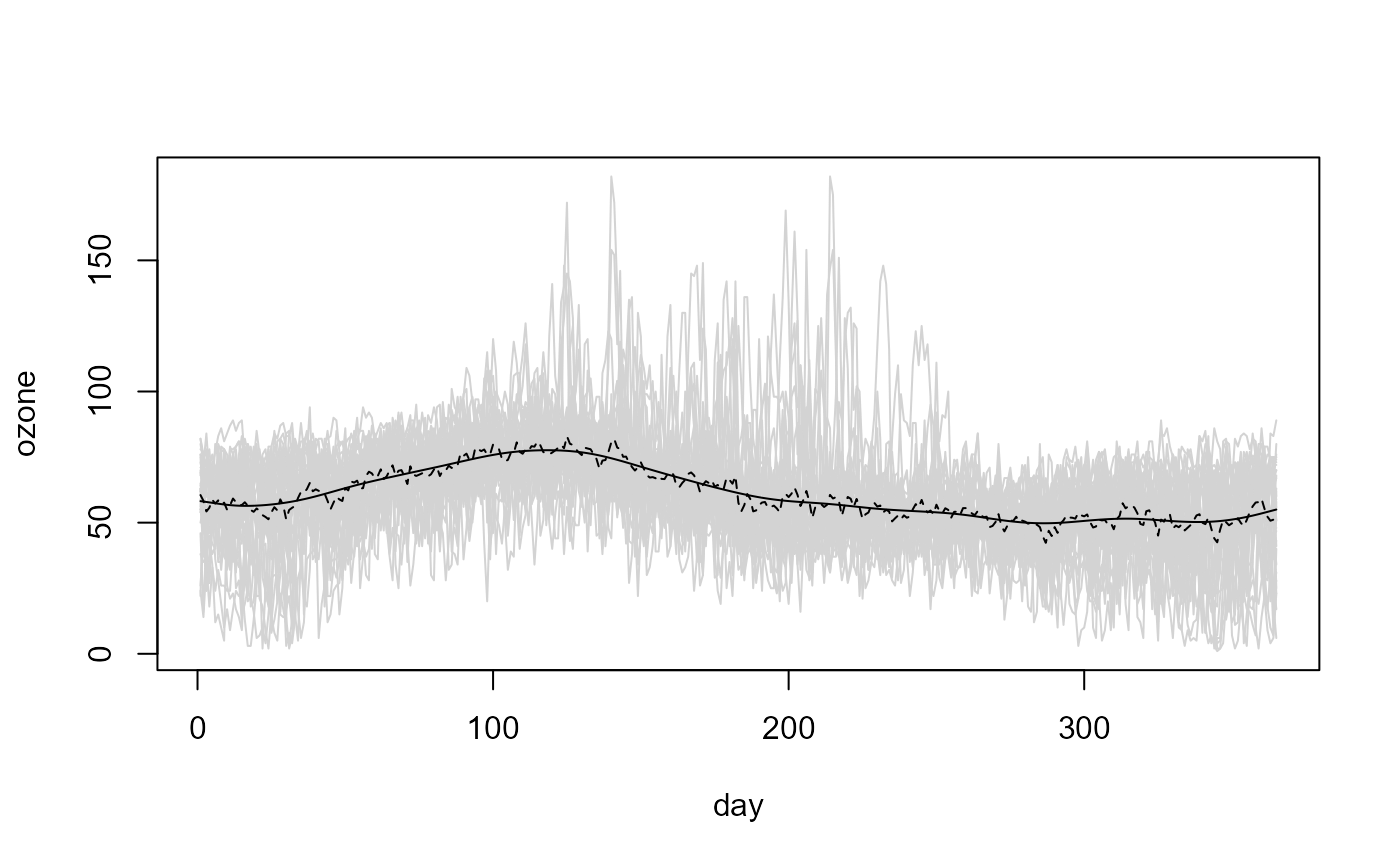
fd <- npf.data(ozone, dimnames = "day")
# Linear Local trend estimate
lp <- locpol(fd, h = 35)
# Plot
plot(fd, col = "lightgray", legend = FALSE)
lines(lp$data$x, lp$biny, lty = 2) # x = coords(fd)
lines(lp$data$x, lp$est)

# Bandwidth selection
# (assuming independence and homoscedasticity)
bin <- npf.binning(fd) # binning
trend.h <- h.cv(bin)$h
trend.h
#>          [,1]
#> [1,] 4.947342
# the selected bandwidth undersmoothes the data...
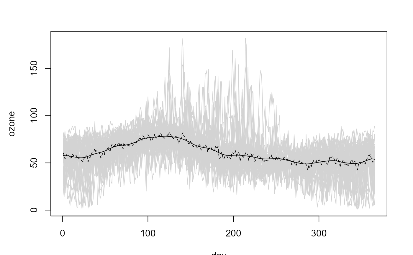
trend.h <- 4*trend.h
# Linear Local trend estimate
lp <- locpol(bin, h = trend.h, hat.bin = TRUE)
# Plot
plot(fd, col = "lightgray", legend = FALSE)
lines(lp$data$x, lp$biny, lty = 2)
lines(lp$data$x, lp$est)