Local polynomial variance estimation

Estimates the functional variance (and its first derivatives) using local polynomial kernel smoothing.

np.var(x, ...)

# S3 method for npf.locpol
np.var(
  x,
  h = NULL,
  degree = 1 + as.numeric(drv),
  drv = FALSE,
  hat.bin = FALSE,
  ncv = 0,
  ...
)

# S3 method for npf.bin.res2
np.var(
  x,
  h = NULL,
  degree = 1 + as.numeric(drv),
  drv = FALSE,
  hat.bin = FALSE,
  ncv = 0,
  ...
)

# S3 method for npf.var
predict(object, newx = NULL, ...)

Arguments

x

an object used to select a method.

...

further arguments passed to or from other methods.

h

(full) bandwidth matrix (controls the degree of smoothing; only the upper triangular part of h is used).

degree

degree of the local polynomial used. Defaults to 1 (local linear estimation).

drv

logical; if TRUE, the matrix of estimated first derivatives is returned.

hat.bin

logical; if TRUE, the hat matrix of the binned data is returned.

ncv

integer; determines the number of cells leaved out in each dimension. Defaults to 0 (the full data is used) and it is not normally changed by the user in this setting. See "Details" below.

object

object used to select a method.

newx

vector with the (irregular) points to predict (interpolate).

Value

Returns an S3 object of class npf.var extending npsp::locpol.bin

(locpol + bin data + grid par.).

If newx == NULL, predict.npf.var returns the variance estimates corresponding to the discretization points (otherwise npsp::interp.data.grid is called).

See also

npf.bin.res2

Examples

fd <- npf.data(ozone, dimnames = "day")
# Linear Local trend estimate
lp <- locpol(fd, h = 35)
# Linear Local variance estimate
lp.var <- np.var(lp, h = 50)
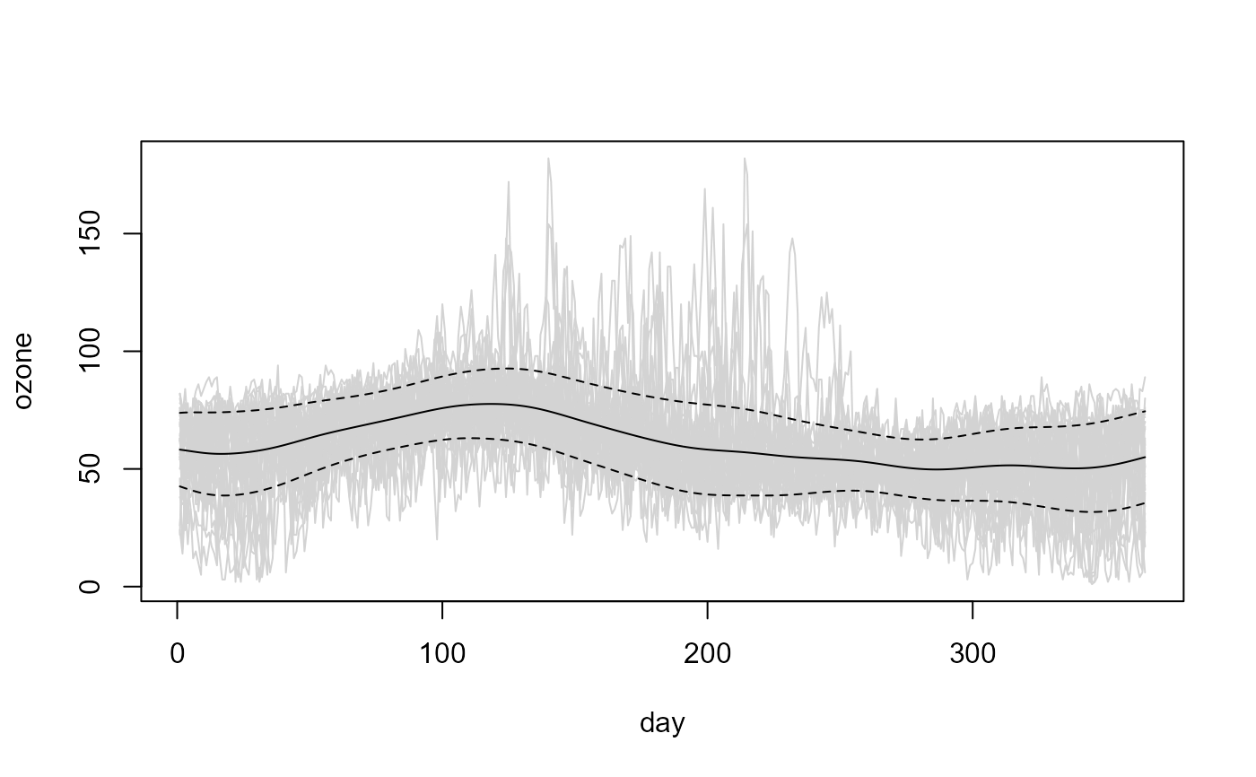
# Plot data + estimated trend -+ estimated std. dev.
plot(lp$data, col = "lightgray", legend = FALSE)
x <- lp$data$x
y <- lp$est
lines(x, y)
matlines(x, y + sqrt(lp.var$est) %o% c(-1, 1), col = 1, lty = 2)

# Bandwidth selection (assuming independence)
bin.res2 <- npf.bin.res2(lp)
var.h <- h.cv(bin.res2)$h
# the selected bandwidth undersmoothes the squared residuals...
var.h <- 7*var.h
# Linear Local variance estimate
lp.var <- np.var(lp, h = var.h)
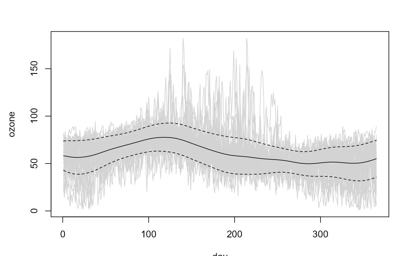
# Plot data + estimated trend -+ estimated std. dev.
plot(lp$data, col = "lightgray", legend = FALSE)
x <- lp$data$x
y <- lp$est
lines(x, y)
matlines(x, y + sqrt(lp.var$est) %o% c(-1, 1), col = 1, lty = 2)