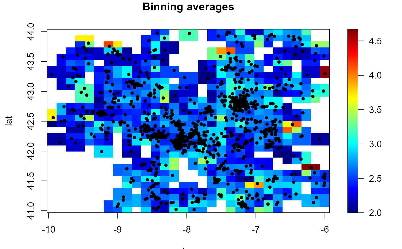
Discretizes the data into a regular grid (computes a binned approximation) using the simple and linear multivariate binning techniques described in Wand (1994).
binning(
  x,
  y = NULL,
  nbin = NULL,
  type = c("linear", "simple"),
  set.NA = FALSE,
  window = NULL,
  ...
)

as.bin.data(object, ...)

# S3 method for class 'data.grid'
as.bin.data(object, data.ind = 1, weights.ind = NULL, ...)

# S3 method for class 'bin.data'
as.bin.data(object, ...)

# S3 method for class 'SpatialGridDataFrame'
as.bin.data(object, data.ind = 1, weights.ind = NULL, ...)
Arguments
- x
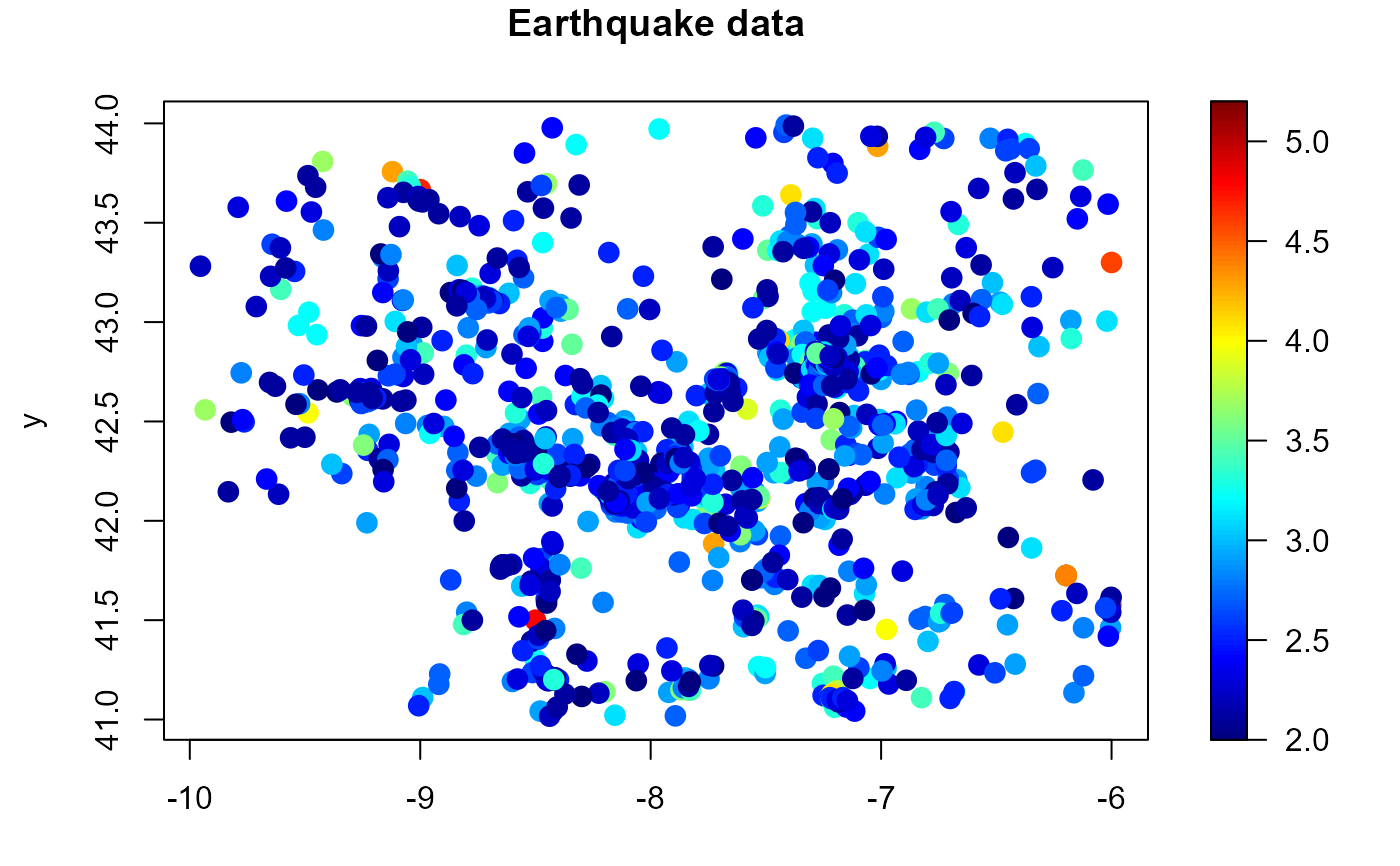
vector or matrix of covariates (e.g. spatial coordinates). Columns correspond with covariates (coordinate dimension) and rows with data.
- y
vector of data (response variable).
- nbin
vector with the number of bins on each dimension.
- type
character, binning method:
"linear"(default) or"simple".- set.NA
logical. If
TRUE, sets the bin averages corresponding to cells without data toNA.- window
spatial window (values outside this window will be masked), currently an sp-object of class extending
SpatialPolygons.- ...
further arguments passed to
mask.bin.data().- object
(gridded data) used to select a method.
- data.ind
integer (or character) with the index (or name) of the component containing the bin averages.
- weights.ind
integer (or character) with the index (or name) of the component containing the bin counts/weights (if not specified, they are set to
as.numeric( is.finite( object[[data.ind]] ))).
Value
If y != NULL, an S3 object of class bin.data (gridded
binned data; extends bin.den) is returned.
A data.grid object with the following 4 components:
- biny
vector or array (dimension
nbin) with the bin averages.- binw
vector or array (dimension
nbin) with the bin counts (weights).- grid
- data
a list with 3 components:
xargumentx.yargumenty.med(weighted) mean of the (binned) data.
If y == NULL, bin.den is called and a
bin.den-class object is returned.
Details
If parameter nbin is not specified is set to pmax(25, rule.binning(x)).
Setting set.NA = TRUE (equivalent to biny[binw == 0] <- NA)
may be useful for plotting the binned averages $biny
(the hat matrix should be handled with care when using locpol).
References
Wand M.P. (1994) Fast Computation of Multivariate Kernel Estimators. Journal of Computational and Graphical Statistics, 3, 433-445.