Cross-validation methods for bandwidth selection

Selects the bandwidth of a local polynomial kernel (regression, density or variogram) estimator using (standart or modified) CV, GCV or MASE criteria.

h.cv(bin, ...)

# S3 method for bin.data
h.cv(
  bin,
  objective = c("CV", "GCV", "MASE"),
  h.start = NULL,
  h.lower = NULL,
  h.upper = NULL,
  degree = 1,
  ncv = ifelse(objective == "CV", 2, 0),
  cov.bin = NULL,
  DEalgorithm = FALSE,
  warn = TRUE,
  tol.mask = npsp.tolerance(2),
  ...
)

# S3 method for bin.den
h.cv(
  bin,
  h.start = NULL,
  h.lower = NULL,
  h.upper = NULL,
  degree = 1,
  ncv = 2,
  DEalgorithm = FALSE,
  ...
)

# S3 method for svar.bin
h.cv(
  bin,
  loss = c("MRSE", "MRAE", "MSE", "MAE"),
  h.start = NULL,
  h.lower = NULL,
  h.upper = NULL,
  degree = 1,
  ncv = 1,
  DEalgorithm = FALSE,
  warn = FALSE,
  ...
)

hcv.data(
  bin,
  objective = c("CV", "GCV", "MASE"),
  h.start = NULL,
  h.lower = NULL,
  h.upper = NULL,
  degree = 1,
  ncv = ifelse(objective == "CV", 1, 0),
  cov.dat = NULL,
  DEalgorithm = FALSE,
  warn = TRUE,
  ...
)

Arguments

bin: object used to select a method (binned data, binned density or binned semivariogram).
...: further arguments passed to or from other methods (e.g. parameters of the optimization routine).
objective: character; optimal criterion to be used ("CV", "GCV" or "MASE").
h.start: vector; initial values for the parameters (diagonal elements) to be optimized over. If DEalgorithm == FALSE (otherwise not used), defaults to (3 + ncv) * lag, where lag = bin$grid$lag.
h.lower: vector; lower bounds on each parameter (diagonal elements) to be optimized. Defaults to (1.5 + ncv) * bin$grid$lag.
h.upper: vector; upper bounds on each parameter (diagonal elements) to be optimized. Defaults to 1.5 * dim(bin) * bin$grid$lag.
degree: degree of the local polynomial used. Defaults to 1 (local linear estimation).
ncv: integer; determines the number of cells leaved out in each dimension. (0 to GCV considering all the data, $>0$ to traditional or modified cross-validation). See "Details" bellow.
cov.bin: (optional) covariance matrix of the binned data or semivariogram model (svarmod-class) of the (unbinned) data. Defaults to the identity matrix.
DEalgorithm: logical; if TRUE, the differential evolution optimization algorithm in package DEoptim is used.
warn: logical; sets the handling of warning messages (normally due to the lack of data in some neighborhoods). If FALSE all warnings are ignored.
tol.mask: tolerance used in the aproximations. Defaults to npsp.tolerance(2).
loss: character; CV error. See "Details" bellow.
cov.dat: covariance matrix of the data or semivariogram model (of class extending svarmod). Defaults to the identity matrix (uncorrelated data).

Value

Returns a list containing the following 3 components:

h: the best (diagonal) bandwidth matrix found.
value: the value of the objective function corresponding to h.
objective: the criterion used.

Details

Currently, only diagonal bandwidths are supported.

h.cv methods use binning approximations to the objective function values (in almost all cases, an averaged squared error). If ncv > 0, estimates are computed by leaving out binning cells with indexes within the intervals $[x_i - ncv + 1, x_i + ncv - 1]$, at each dimension i, where $x$ denotes the index of the estimation location. $ncv = 1$ corresponds with traditional cross-validation and $ncv > 1$ with modified CV (it may be appropriate for dependent data; see e.g. Chu and Marron, 1991, for the one dimensional case). Setting ncv >= 2 would be recommended for sparse data (as linear binning is used). For standard GCV, set ncv = 0 (the whole data would be used). For theoretical MASE, set bin = binning(x, y = trend.teor), cov = cov.teor and ncv = 0.

If DEalgorithm == FALSE, the "L-BFGS-B" method in optim is used.

The different options for the argument loss in h.cv.svar.bin() define the CV error considered in semivariogram estimation:

"MSE": Mean squared error
"MRSE": Mean relative squared error
"MAE": Mean absolute error
"MRAE": Mean relative absolute error

hcv.data evaluates the objective function at the original data (combining a binning approximation to the nonparametric estimates with a linear interpolation), this can be very slow (and memory demanding; consider using h.cv instead). If ncv > 1 (modified CV), a similar algorithm to that in h.cv is used, estimates are computed by leaving out binning cells with indexes within the intervals $[x_i - ncv + 1, x_i + ncv - 1]$.

References

Chu, C.K. and Marron, J.S. (1991) Comparison of Two Bandwidth Selectors with Dependent Errors. The Annals of Statistics, 19, 1906-1918.

Francisco-Fernandez M. and Opsomer J.D. (2005) Smoothing parameter selection methods for nonparametric regression with spatially correlated errors. Canadian Journal of Statistics, 33, 539-558.

Examples

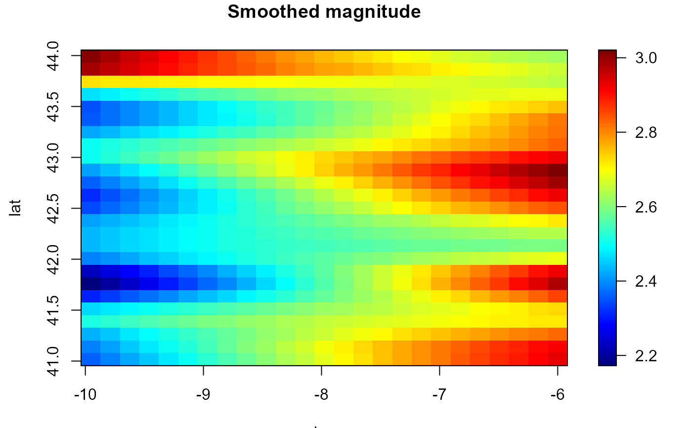
# Trend estimation
bin <- binning(earthquakes[, c("lon", "lat")], earthquakes$mag)
hcv <- h.cv(bin, ncv = 2)
lp <- locpol(bin, h = hcv$h)
# Alternatively, `locpolhcv()` could be called instead of the previous code. 

simage(lp, main = 'Smoothed magnitude')
contour(lp, add = TRUE)
with(earthquakes, points(lon, lat, pch = 20))


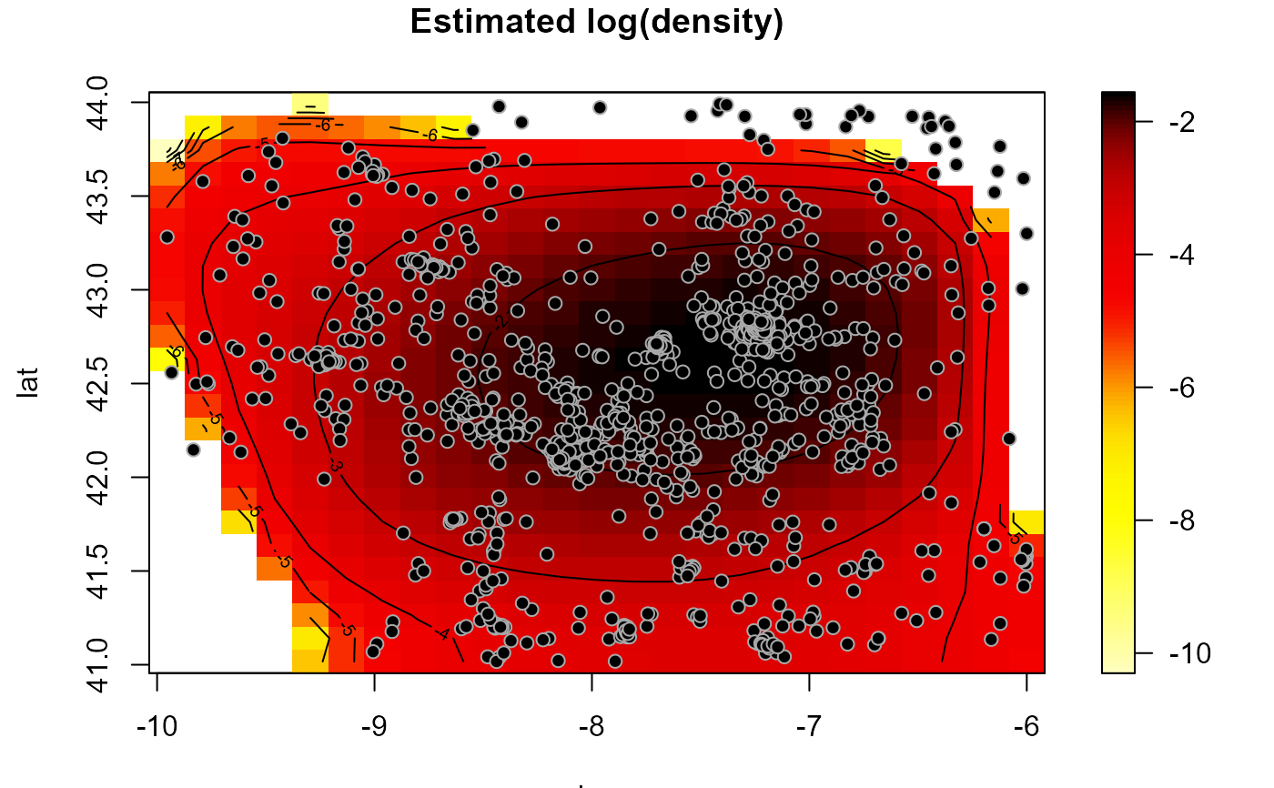
# Density estimation
hden <- h.cv(as.bin.den(bin))
den <- np.den(bin, h = hden$h)

plot(den, main = 'Estimated log(density)')