Introduction to the npsp Package

This vignette (a working draft) tries to illustrate the use of the npsp (Nonparametric spatial statistics) package. This package implements nonparametric methods for inference on multidimensional geostatistical processes, avoiding the misspecification problems that may arise when using parametric models. The spatial process can be either stationary or show a non-constant trend. Joint estimation of the trend and the semivariogram can be performed automatically, by using the function np.fitgeo(), or by a step-by-step approach.

Introduction

We will assume that $\left\{ Y(\mathbf{x}),\mathbf{x}\in D \subset \mathbb{R}^{d}\right\}$ is a spatial process that can be modeled as: $Y(\mathbf{x})=\mu(\mathbf{x})+\varepsilon(\mathbf{x}),$

where $\mu(\cdot)$ is the trend function (large-scale variation) and the error term $\varepsilon$ (small-scale variation), is a second order stationary process with zero mean and covariogram $C(\mathbf{u}) = Cov(\varepsilon \left( \mathbf{x}\right) ,\varepsilon \left(\mathbf{x}+\mathbf{u}\right) )$ , with $\mathbf{u} \in D$ .

In this framework, given $n$ observed values $\mathbf{Y}=( Y(\mathbf{x}_{1}),...,Y(\mathbf{x}_{n}))^{t}$ , the first step consists in estimate the trend $\mu(\mathbf{x})$ and the semivariogram $\gamma(\mathbf{h}) = C(\mathbf{0}) - C(\mathbf{u})$ .

There are several R packages, such as gstat or geoR, which implement the traditional geostatistical techniques to approximate these functions. Nevertheless, as these approaches usually assume parametric models, they can present misspecification problems.

The aim of the npsp package is to provide nonparametric tools for geostatistical modeling and interpolation, under the general spatial model (large + small variation scales), and without assuming any specific form (parametric model) for the trend and the variogram of the process.

library(npsp)

##  Package npsp: Nonparametric Spatial Statistics,
##  version 0.7-14 (built on 2024-07-09).
##  Copyright (C) R. Fernandez-Casal 2012-2024.
##  Type `help(npsp)` for an overview of the package or
##  visit https://rubenfcasal.github.io/npsp.

The precipitation data set (sp::SpatialGridDataFrame class object), supplied with the npsp package, will be used in the examples in this work. The data consist of total precipitations (square-root of rainfall inches) during March 2016 recorded over 1053 locations on the continental part of USA.

library(sp)
summary(precipitation)

## Object of class SpatialPointsDataFrame
## Coordinates:
##         min      max
## x1 -124.555 -67.7928
## x2   24.555  48.9676
## Is projected: FALSE 
## proj4string : [+proj=longlat +ellps=WGS84]
## Number of points: 1053
## Data attributes:
##        y              WBAN                 state     
##  Min.   :0.000   Min.   :  166   USA          :1053  
##  1st Qu.:1.100   1st Qu.:13733   Alaska       :   0  
##  Median :1.539   Median :23254   Isla Hawai   :   0  
##  Mean   :1.551   Mean   :39700   Isla Honolulu:   0  
##  3rd Qu.:1.954   3rd Qu.:63895   Isla Kauai   :   0  
##  Max.   :4.105   Max.   :94996   Isla Maui    :   0  
##                                  (Other)      :   0

For instance, spoints() function may be used to plot the data…

spoints(precipitation)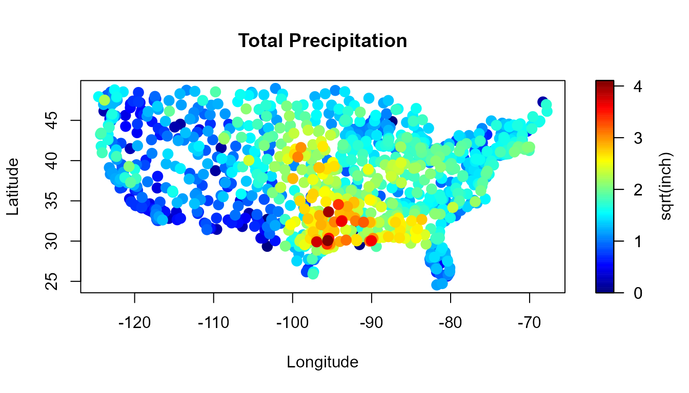

Function scattersplot() may be used to detect the presence of a non-constant trend…

scattersplot(precipitation)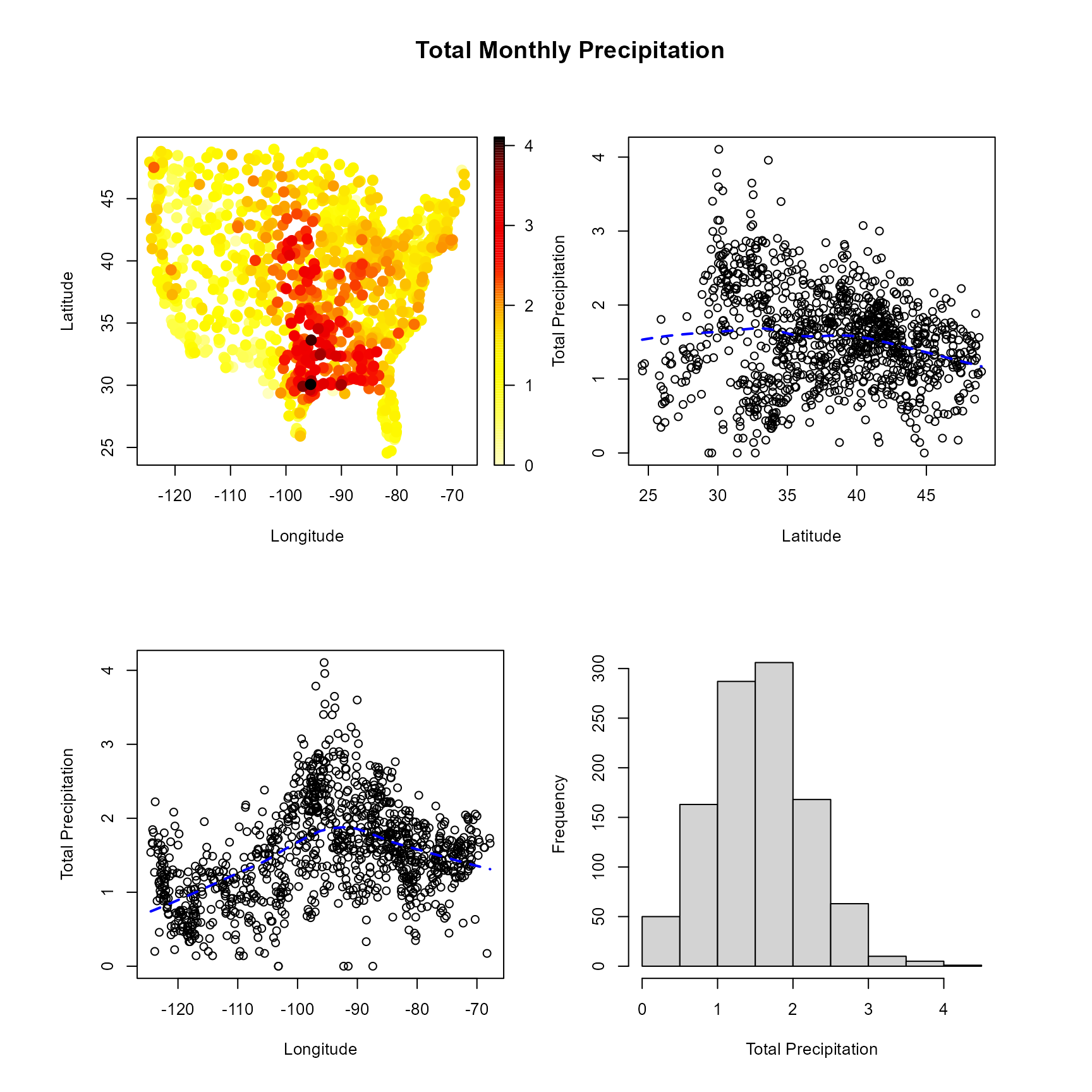

Trend estimation

The local polynomial trend estimator $\hat{\mu}_{\mathbf{H}}(\mathbf{x})$ (e.g. Fan and Gijbels, 1996), obtained by polynomial smoothing of $\{(\mathbf{x}_{i},Y(\mathbf{x}_{i})):i=1,\ldots,n\}$ , is the solution for $\beta_0$ to the least squares minimization problem $\begin{aligned} \min_{\beta_0 ,\boldsymbol{\beta}_1, \ldots, \boldsymbol{\beta}_p} \sum_{i=1}^{n}\left\{ Y(\mathbf{x}_{i})-\beta_0 -\boldsymbol{\beta}_1^{t}(\mathbf{x}_{i}-\mathbf{x}) - \ldots \right. \nonumber \\ \left. -\boldsymbol{\beta}_p^{t}(\mathbf{x}_{i}-\mathbf{x})^p \right\}^{2} K_{\mathbf{H}}(\mathbf{x}_{i}-\mathbf{x}), \end{aligned}$ where $\mathbf{H}$ is a $d\times d$ symmetric positive definite matrix; $K$ is a $d$ -dimensional kernel and $K_{\mathbf{H}}(\mathbf{u})=\left\vert \mathbf{H}\right\vert ^{-1}K(\mathbf{H}^{-1}\mathbf{u})$ .

The bandwidth matrix $\mathbf{H}$ controls the shape and size of the local neighborhood used to estimate $\mu(\mathbf{x})$ .

The local trend estimates can be computed in practice with the locpol() function. A full bandwidth matrix and a multiplicative triweight kernel is used to compute the weights. Main calculations are performed in Fortran using the LAPACK library.

x <- coordinates(precipitation)
y <- precipitation$y
lp <- locpol(x, y, nbin = c(120, 120), h = diag(c(5, 5)))

We can plot the trend estimates with function simage() (or spersp()). Additionally, in this case the estimates outside of continental part of USA will be masked.

attr <- attributes(precipitation)
border <- attr$border 
# Mask grid points outside of continental part of USA
lp <- mask(lp, window = border)

## Warning in mask.locpol.bin(lp, window = border): 
## some data will be masked...

interior <- attr$interior 
slim <- range(y)
col <- jet.colors(256)
simage(lp,  slim = slim, main = "Trend estimates",
       col = col, xlab = "Longitude", ylab = "Latitude", asp = 1)
plot(border, border = "darkgray", lwd = 2, add = TRUE)
plot(interior, border = "lightgray", lwd = 1, add = TRUE)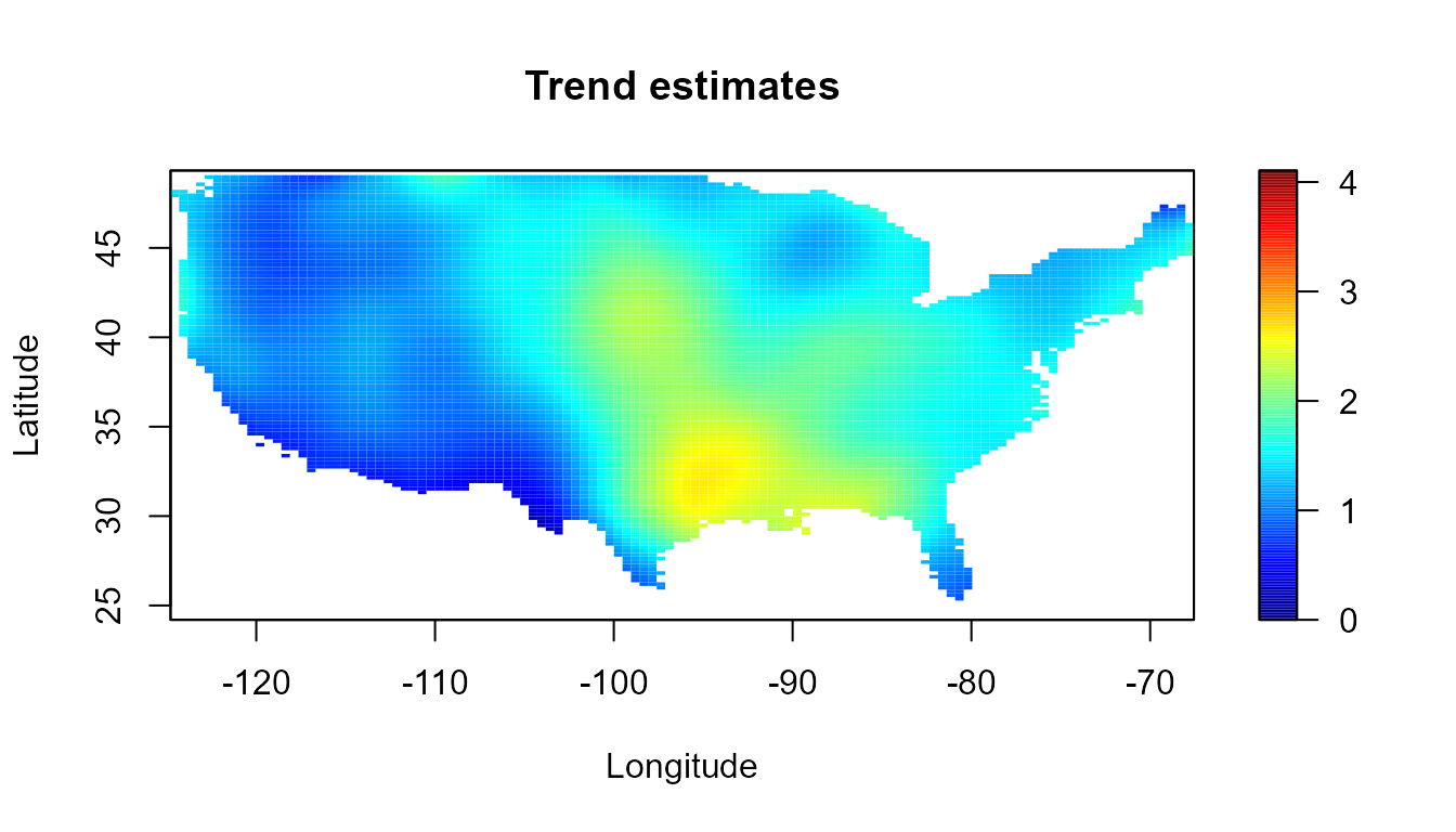

The smoothing procedures in npsp use linear binning to discretize the data. For instance, instead of the previous code we can use:

bin <- binning(x, y, nbin = c(120, 120), window = border)
# lp <- locpol(bin, h = diag(c(5, 5)))
lp2 <- locpol(bin, h = diag(c(2, 2)))
simage(lp2, slim = slim, main = "Trend estimates",
       col = col, xlab = "Longitude", ylab = "Latitude", asp = 1)
plot(border, border = "darkgray", lwd = 2, add = TRUE)
plot(interior, border = "lightgray", lwd = 1, add = TRUE)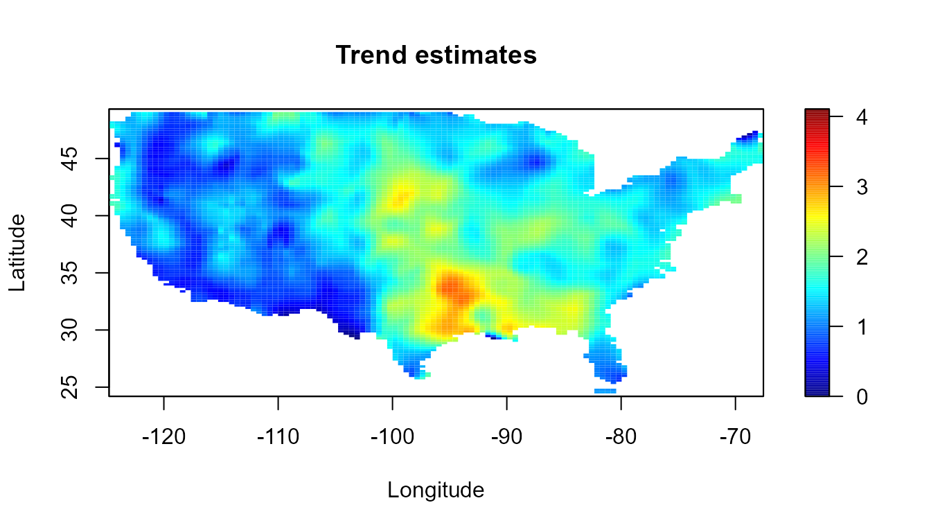

Usually two grids will be considered, a low resolution one to speed up computations during the modeling (e.g. by using the default values), and a higher resolution one to obtain the final results.

Bandwidth selection

The trend estimates depends crucially on the bandwidth matrix $H$ . A small bandwidth will produce undersmoothed estimates, whereas a big bandwidth will oversmooth the data. Although it may be subjectively choosed by eye, it could be very beneficial to have automatic selection criteria from the data.

Traditional bandwidth selectors, such as cross validation (CV) or generalized cross validation (GCV), do not have a good performance for dependent data (Opsomer et al, 2001), since they tend to undersmooth the trend function.

The modified cross-validation criteria (MCV), proposed in (Chu and Marron, 1991) for time series, can be adapted for spatial data, by ignoring observations in a neighbourhood $N(i)$ around $\mathbf{x}_{i}$ . Note that the ordinary CV approach is a particular case with $N(i)=\left\lbrace \mathbf{x}_{i} \right\rbrace$ .

In practice, the bandwidth can be selected through the h.cv() (or hcv.data()) function.

bin <- binning(x, y, window = border)
lp0.h <- h.cv(bin)$h
lp0 <- locpol(bin, h = lp0.h, hat.bin = TRUE)

An alternative is the corrected generalized cross-validation criterion (CGCV), proposed in Francisco-Fernández and Opsomer (2005), that takes the spatial dependence into account. To use this approach in practice (by setting objective = "GCV" and cov.bin in h.cv), an estimate of the variogram is previously required.

Variogram estimation

When the process is assumed stationary, the pilot local linear estimate $\hat\gamma(\mathbf{u})$ is obtained by the linear smoothing of $\left(\mathbf{x}_{i}-\mathbf{x}_{j},(Y(\mathbf{x}_i)- Y(\mathbf{x}_j))^2/2 \right)$ . The corresponding bandwidth can be selected, for instance, by minimizing the cross-validation relative squared error.

In the general setting with a non constant trend, the natural approach consists in removing the trend and estimating the variogram from the residuals $\mathbf{r}=\mathbf{Y}-\mathbf{SY}$ . Nevertheless, the residuals variability may be very different to that of the true errors (see e.g. Cressie, 1993, Section 3.4.3, for the case of the linear trend estimator). As the bias due to the direct use of residuals in variogram estimation may have a significant impact on inference, a similar approach to that described in Fernández-Casal and Francisco-Fernández (2014) could be considered.

In practice, the local linear variogram estimates can be computed with functions np.svar() and np.svariso.corr(). The generic function h.cv() may be used to select the corresponding bandwidth.

svar.bin <- svariso(x, residuals(lp0), nlags = 60, maxlag = 20)  
svar.h <- h.cv(svar.bin)$h

svar.np <- np.svar(svar.bin, h = svar.h)
svar.np2 <- np.svariso.corr(lp0, nlags = 60, maxlag = 20, 
                            h = svar.h, plot = FALSE)

The final variogram estimate is obtained by fitting a “nonparametric” isotropic Shapiro-Botha variogram model (Shapiro and Botha, 1991), to the nonparametric pilot estimate, by using the function fitsvar.sb.iso().

svm0 <- fitsvar.sb.iso(svar.np, dk = 0) 
svm1 <- fitsvar.sb.iso(svar.np2, dk = 0) 
# plot...
plot(svm1, main = "Nonparametric bias-corrected semivariogram\nand fitted models", 
     legend = FALSE, xlim = c(0,max(coords(svar.np2))), 
     ylim = c(0,max(svar.np2$biny, na.rm = TRUE)))
plot(svm0, lwd = c(1, 1), add = TRUE)
plot(svar.np, type = "p", pch = 2, add = TRUE)
# abline(h = c(svm1$nugget, svm1$sill), lty = 3)
# abline(v = 0, lty = 3)
legend("bottomright", legend = c("corrected", 'biased'),
            lty = c(1, 1), pch = c(1, 2), lwd = c(1, 1))

Automatic modeling

Function np.fitgeo() implements an automatic procedure for the joint estimation of the trend and the semivariogram. The algorithm is as follows:

Select an initial bandwidth to estimate the trend using the MCV criterion (function h.cv()).
Compute the local linear trend estimate (function locpol()).
Obtain a bias-corrected pilot semivariogram estimate from the corresponding residuals (function np.svariso.corr()).
Fit a valid Shapiro-Botha model to the pilot semivariogram estimates (function fitsvar.sb.iso()).
Select a new bandwidth matrix for trend estimation with the CGCV criterion, using the fitted variogram model to approximate the data covariance matrix (function h.cv() with objective = "GCV" and cov.bin = fitted variogram model).
Repeat steps 2-5 until convergence (in practice, only two iterations are usually needed).

geomod <- np.fitgeo(x, y, nbin = c(30, 30), maxlag = 20, svm.resid = TRUE, window = border)
plot(geomod)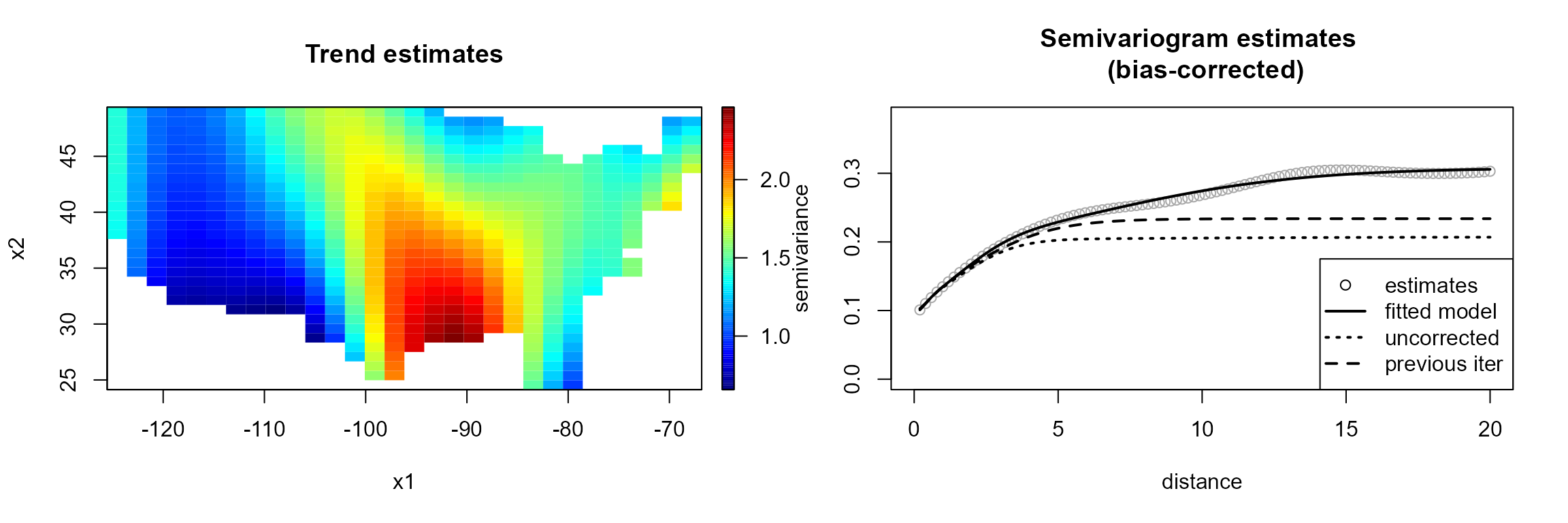

Setting corr.svar = TRUE may be very slow (and memory demanding) when the number of data is large (note also that the bias in the residual variogram decreases when the sample size increases).

Kriging

The final trend and variogram estimates could be employed for spatial prediction, by using method np.kriging().

krig.grid <- np.kriging(geomod, ngrid = c(120, 120))
# Plot kriging predictions and kriging standard deviations
old.par <- par(mfrow = c(1,2), omd = c(0.0, 0.98, 0.0, 1))
simage(krig.grid, 'kpred', main = 'Kriging predictions', slim = slim,
      xlab = "Longitude", ylab = "Latitude" , col = col, asp = 1, reset = FALSE)
plot(border, border = "darkgray", lwd = 2, add = TRUE)
plot(interior, border = "lightgray", lwd = 1, add = TRUE)
simage(krig.grid, 'ksd', main = 'Kriging sd', xlab = "Longitude", 
       ylab = "Latitude" , col = hot.colors(256), asp = 1, reset = FALSE)
plot(border, border = "darkgray", lwd = 2, add = TRUE)
plot(interior, border = "lightgray", lwd = 1, add = TRUE)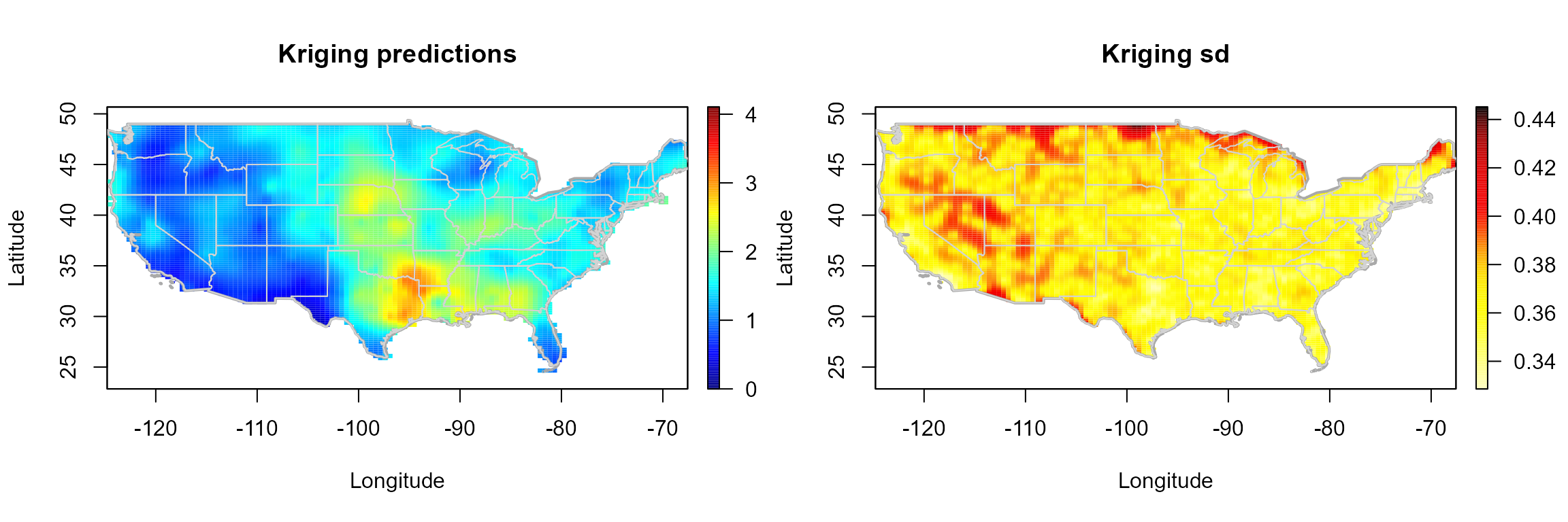

par(old.par)

Currently, only global residual kriging is implemented. Users are encouraged to use gstat::krige() (or krige.cv()) together with as.vgm() for local kriging (see e.g. https://rubenfcasal.github.io/npsp/articles/krigstat.html).

Conclusions and future work

Unlike traditional geostatistical methods, the nonparametric procedures avoid problems due to model misspecification.

The bias due to the direct use of residuals, may have a significant impact on variogram estimation (and consequently on the selected bandwidth with the CGCV criterion). Therefore, the use of the bias-corrected nonparametric variogram estimator would be recommended.

Currently, only isotropic semivariogram estimation is supported, but the intention is to extend this approach to anisotropy in two components (Fernández-Casal et al., 2003), which could be suitable for modeling spatio-temporal dependency.

The nonparametric trend and variogram estimates also allow to perform inferences about other characteristics of interest of the process, for instance, by using the bootstrap algorithm described in (Castillo-Páez et al., 2019), which will be implemented in the next version of the package (https://github.com/rubenfcasal/npsp).

Acknowledgments

This research has been supported by MINECO grant MTM2017-82724-R, and by the Xunta de Galicia (Grupos de Referencia Competitiva ED431C-2020-14 and Centro de Investigación del Sistema universitario de Galicia ED431G 2019/01), all of them through the ERDF.

References

Castillo-Páez, S., Fernández-Casal, R., García-Soidán, P. (2019). A nonparametric bootstrap method for spatial data. Comput. Stat. Data An., 137, 1–15.

Chu, C. K. and Marron, J. S. (1991). Comparison of Two Bandwidth Selectors with Dependent Errors. The Annals of Statistics 19, 1906–1918.

Cressie, N. (1993). Statistics for Spatial Data. Wiley, New York.

Fernández-Casal, R. (2019). npsp: Nonparametric Spatial Statistics. R package version 0.7-5. https://github.com/rubenfcasal/npsp.

Fan, J. and Gijbels, I. (1996). Local polynomial modelling and its applications. Chapman & Hall, London.

Fernández-Casal, R. and Francisco-Fernández, M. (2014). Nonparametric bias-corrected variogram estimation under non-constant trend. Stochastic Environmental Research and Risk Assessment 28, 1247–1259.

Fernández-Casal, R., González Manteiga, W. and Febrero-Bande, M. (2003). Flexible Spatio-Temporal Stationary Variogram Models. Statistics and Computing 13, 127–136.

Francisco-Fernández, M. and Opsomer, J. D. (2005). Smoothing parameter selection methods for nonparametric regression with spatially correlated errors. The Canadian Journal of Statistics 33, 279–295.

Opsomer, J. D., Wang, Y. and Yang, Y. (2001). Nonparametric regression with correlated errors. Statistical Science 16, 134–153.

Shapiro, A. and Botha, J.D. (1991). Variogram fitting with a general class of conditionally non-negative definite functions. Computational Statistics and Data Analysis 11, 87–96.

Ruben Fernandez-Casal (ruben.fcasal@udc.es)

npsp 0.7.14