6.3 Regresión y correlación
6.3.1 Regresión lineal simple
Utilizando la función lm (modelo lineal) se puede llevar a cabo, entre otras muchas cosas, una regresión lineal simple
lm(satisfac ~ fidelida, data = hatco)##
## Call:
## lm(formula = satisfac ~ fidelida, data = hatco)
##
## Coefficients:
## (Intercept) fidelida
## 1.6074 0.0685modelo <- lm(satisfac ~ fidelida, data = hatco, na.action=na.exclude)
summary(modelo)##
## Call:
## lm(formula = satisfac ~ fidelida, data = hatco, na.action = na.exclude)
##
## Residuals:
## Min 1Q Median 3Q Max
## -1.47492 -0.37341 0.09358 0.38258 1.25258
##
## Coefficients:
## Estimate Std. Error t value Pr(>|t|)
## (Intercept) 1.607399 0.322436 4.985 2.71e-06 ***
## fidelida 0.068500 0.006848 10.003 < 2e-16 ***
## ---
## Signif. codes: 0 '***' 0.001 '**' 0.01 '*' 0.05 '.' 0.1 ' ' 1
##
## Residual standard error: 0.6058 on 97 degrees of freedom
## (1 observation deleted due to missingness)
## Multiple R-squared: 0.5078, Adjusted R-squared: 0.5027
## F-statistic: 100.1 on 1 and 97 DF, p-value: < 2.2e-16plot(hatco$fidelida, hatco$satisfac) # Cuidado con el orden de las variables
# with(hatco, plot(fidelida, satisfac)) # Alternativa empleando with
# plot(satisfac ~ fidelida, data = hatco) # Alternativa empleando fórmulas
abline(modelo)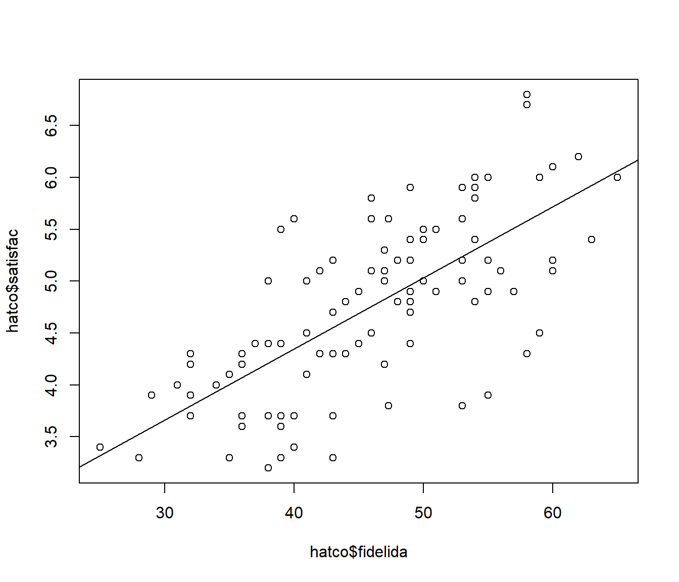
Valores ajustados
fitted(modelo)## 1 2 3 4 5 6 7 8
## 3.799412 4.552917 4.895419 3.799412 5.580423 4.689918 4.758418 4.621417
## 9 10 11 12 13 14 15 16
## 5.922925 5.306421 3.799412 4.826919 4.278915 4.210415 5.306421 4.963919
## 17 18 19 20 21 22 23 24
## 4.210415 4.347416 5.306421 5.374922 4.415916 4.004913 5.374922 4.073414
## 25 26 27 28 29 30 31 32
## 4.963919 4.963919 4.073414 5.306421 4.963919 4.758418 4.552917 5.237921
## 33 34 35 36 37 38 39 40
## 5.717424 4.847469 4.004913 4.278915 4.621417 4.758418 3.593911 3.525410
## 41 42 43 44 45 46 47 48
## 4.347416 5.580423 5.237921 4.895419 4.210415 5.306421 5.374922 4.552917
## 49 50 51 52 53 54 55 56
## 5.511923 5.237921 4.415916 5.237921 5.032420 3.799412 4.278915 4.826919
## 57 58 59 60 61 62 63 64
## 5.854425 6.059926 4.758418 5.032420 5.306421 5.717424 4.826919 4.073414
## 65 66 67 68 69 70 71 72
## 4.347416 4.689918 5.648924 4.758418 5.580423 4.963919 5.032420 5.374922
## 73 74 75 76 77 78 79 80
## 5.100920 5.717424 4.415916 4.963919 4.484416 4.826919 4.278915 5.443422
## 81 82 83 84 85 86 87 88
## 5.648924 4.847469 4.415916 4.141914 5.237921 4.552917 5.100920 4.073414
## 89 90 91 92 93 94 95 96
## 3.936413 5.717424 4.963919 4.278915 4.552917 4.073414 3.730912 3.319909
## 97 98 99 100
## 5.717424 4.210415 4.484416 NAResiduos
head(resid(modelo))## 1 2 3 4 5 6
## 0.4005878 -0.2529168 0.3045811 0.1005878 1.2195769 -0.2899177qqnorm(resid(modelo))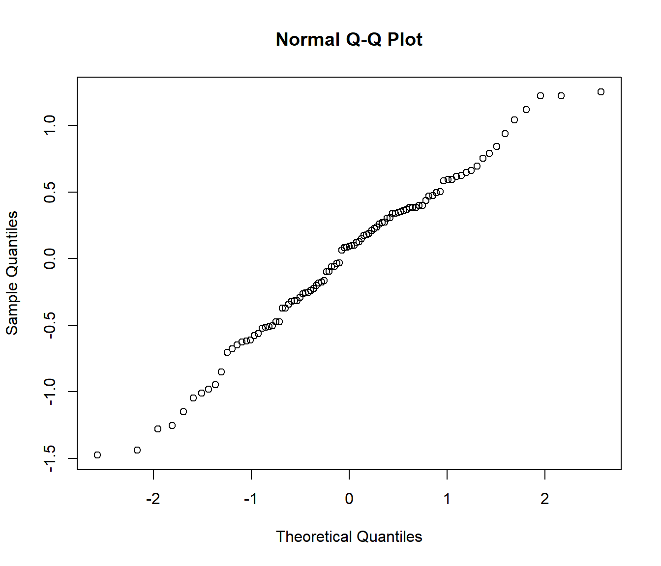
shapiro.test(resid(modelo))##
## Shapiro-Wilk normality test
##
## data: resid(modelo)
## W = 0.98515, p-value = 0.3325plot(hatco$fidelida, hatco$satisfac)
abline(modelo)
# segments(hatco$fidelida, fitted(modelo), hatco$fidelida, hatco$satisfac)
with(hatco, segments(fidelida, fitted(modelo), fidelida, satisfac))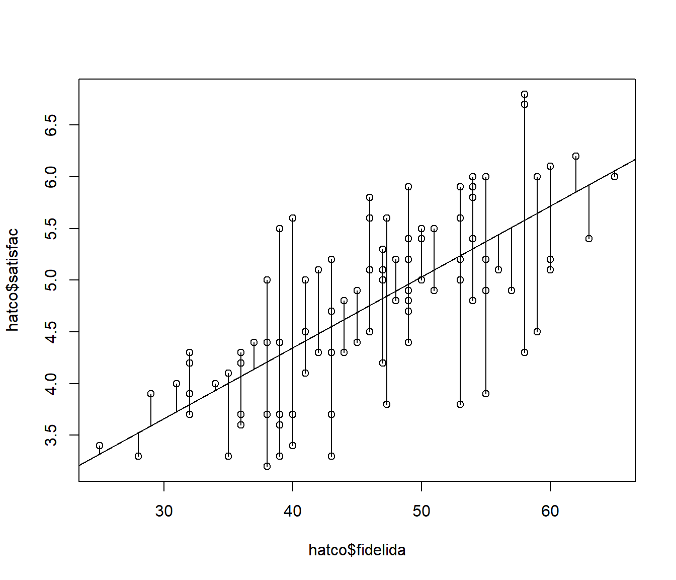
plot(fitted(modelo), resid(modelo))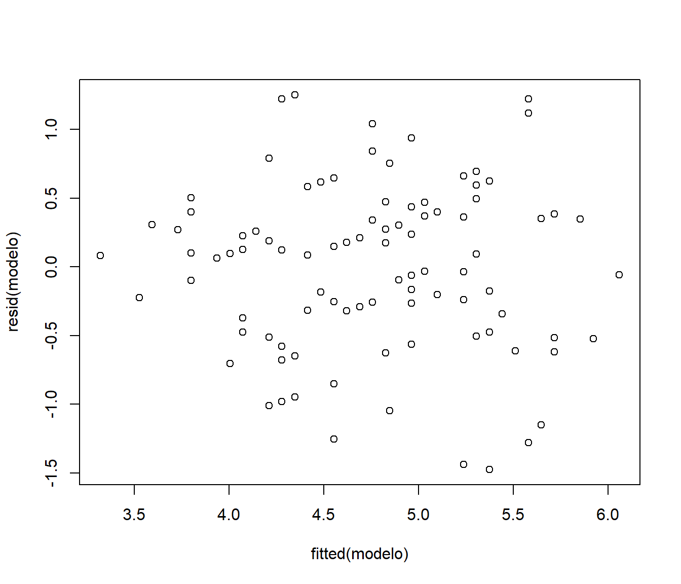
Banda de confianza
predict(modelo, interval='confidence')## fit lwr upr
## 1 3.799412 3.571263 4.027561
## 2 4.552917 4.424306 4.681528
## 3 4.895419 4.772225 5.018613
## 4 3.799412 3.571263 4.027561
## 5 5.580423 5.380031 5.780815
## 6 4.689918 4.567906 4.811929
## 7 4.758418 4.637529 4.879307
## 8 4.621417 4.496801 4.746033
## 9 5.922925 5.665048 6.180803
## 10 5.306421 5.146011 5.466832
## 11 3.799412 3.571263 4.027561
## 12 4.826919 4.705631 4.948206
## 13 4.278915 4.123089 4.434741
## 14 4.210415 4.045670 4.375159
## 15 5.306421 5.146011 5.466832
## 16 4.963919 4.837379 5.090459
## 17 4.210415 4.045670 4.375159
## 18 4.347416 4.199793 4.495038
## 19 5.306421 5.146011 5.466832
## 20 5.374922 5.205264 5.544580
## 21 4.415916 4.275658 4.556174
## 22 4.004913 3.810147 4.199680
## 23 5.374922 5.205264 5.544580
## 24 4.073414 3.889113 4.257714
## 25 4.963919 4.837379 5.090459
## 26 4.963919 4.837379 5.090459
## 27 4.073414 3.889113 4.257714
## 28 5.306421 5.146011 5.466832
## 29 4.963919 4.837379 5.090459
## 30 4.758418 4.637529 4.879307
## 31 4.552917 4.424306 4.681528
## 32 5.237921 5.086103 5.389740
## 33 5.717424 5.494745 5.940103
## 34 4.847469 4.725765 4.969172
## 35 4.004913 3.810147 4.199680
## 36 4.278915 4.123089 4.434741
## 37 4.621417 4.496801 4.746033
## 38 4.758418 4.637529 4.879307
## 39 3.593911 3.330292 3.857530
## 40 3.525410 3.249642 3.801179
## 41 4.347416 4.199793 4.495038
## 42 5.580423 5.380031 5.780815
## 43 5.237921 5.086103 5.389740
## 44 4.895419 4.772225 5.018613
## 45 4.210415 4.045670 4.375159
## 46 5.306421 5.146011 5.466832
## 47 5.374922 5.205264 5.544580
## 48 4.552917 4.424306 4.681528
## 49 5.511923 5.322196 5.701650
## 50 5.237921 5.086103 5.389740
## 51 4.415916 4.275658 4.556174
## 52 5.237921 5.086103 5.389740
## 53 5.032420 4.901205 5.163635
## 54 3.799412 3.571263 4.027561
## 55 4.278915 4.123089 4.434741
## 56 4.826919 4.705631 4.948206
## 57 5.854425 5.608471 6.100378
## 58 6.059926 5.777748 6.342104
## 59 4.758418 4.637529 4.879307
## 60 5.032420 4.901205 5.163635
## 61 5.306421 5.146011 5.466832
## 62 5.717424 5.494745 5.940103
## 63 4.826919 4.705631 4.948206
## 64 4.073414 3.889113 4.257714
## 65 4.347416 4.199793 4.495038
## 66 4.689918 4.567906 4.811929
## 67 5.648924 5.437531 5.860316
## 68 4.758418 4.637529 4.879307
## 69 5.580423 5.380031 5.780815
## 70 4.963919 4.837379 5.090459
## 71 5.032420 4.901205 5.163635
## 72 5.374922 5.205264 5.544580
## 73 5.100920 4.963837 5.238003
## 74 5.717424 5.494745 5.940103
## 75 4.415916 4.275658 4.556174
## 76 4.963919 4.837379 5.090459
## 77 4.484416 4.350544 4.618289
## 78 4.826919 4.705631 4.948206
## 79 4.278915 4.123089 4.434741
## 80 5.443422 5.263964 5.622881
## 81 5.648924 5.437531 5.860316
## 82 4.847469 4.725765 4.969172
## 83 4.415916 4.275658 4.556174
## 84 4.141914 3.967647 4.316181
## 85 5.237921 5.086103 5.389740
## 86 4.552917 4.424306 4.681528
## 87 5.100920 4.963837 5.238003
## 88 4.073414 3.889113 4.257714
## 89 3.936413 3.730815 4.142011
## 90 5.717424 5.494745 5.940103
## 91 4.963919 4.837379 5.090459
## 92 4.278915 4.123089 4.434741
## 93 4.552917 4.424306 4.681528
## 94 4.073414 3.889113 4.257714
## 95 3.730912 3.491126 3.970697
## 96 3.319909 3.006980 3.632839
## 97 5.717424 5.494745 5.940103
## 98 4.210415 4.045670 4.375159
## 99 4.484416 4.350544 4.618289
## 100 NA NA NABanda de predicción
head(predict(modelo, interval='prediction'))## fit lwr upr
## 1 3.799412 2.575563 5.023261
## 2 4.552917 3.343663 5.762171
## 3 4.895419 3.686729 6.104109
## 4 3.799412 2.575563 5.023261
## 5 5.580423 4.361444 6.799403
## 6 4.689918 3.481348 5.898487Representación gráfica de las bandas
bandas.frame <- data.frame(fidelida=24:66)
bc <- predict(modelo, interval = 'confidence', newdata = bandas.frame)
bp <- predict(modelo, interval = 'prediction', newdata = bandas.frame)
plot(hatco$fidelida, hatco$satisfac, ylim = range(hatco$satisfac, bp, na.rm = TRUE))
matlines(bandas.frame$fidelida, bc, lty=c(1,2,2), col='black')
matlines(bandas.frame$fidelida, bp, lty=c(0,3,3), col='red')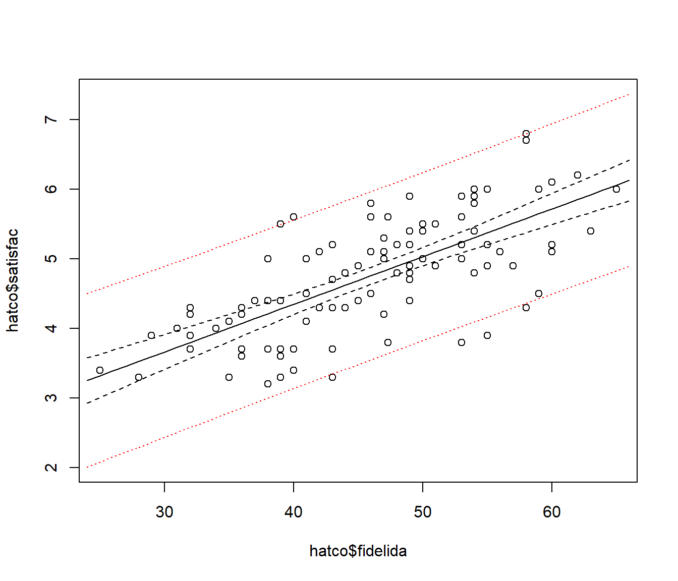
6.3.2 Correlación
Coeficiente de correlación de Pearson
cor(hatco$fidelida, hatco$satisfac, use='complete.obs')## [1] 0.712581cor(hatco[,6:14], use='complete.obs')## velocida precio flexprec imgfabri servconj
## velocida 1.00000000 -0.35439461 0.51879732 0.04885481 0.60908594
## precio -0.35439461 1.00000000 -0.48550163 0.27150666 0.51134698
## flexprec 0.51879732 -0.48550163 1.00000000 -0.11472112 0.07496499
## imgfabri 0.04885481 0.27150666 -0.11472112 1.00000000 0.29800272
## servconj 0.60908594 0.51134698 0.07496499 0.29800272 1.00000000
## imgfvent 0.08084452 0.18873090 -0.03801323 0.79015164 0.24641510
## calidadp -0.48984768 0.46822563 -0.44542562 0.19904126 -0.06152068
## fidelida 0.67428681 0.07682487 0.57807750 0.22442574 0.69802972
## satisfac 0.64981476 0.02636286 0.53057615 0.47553688 0.63054720
## imgfvent calidadp fidelida satisfac
## velocida 0.08084452 -0.48984768 0.67428681 0.64981476
## precio 0.18873090 0.46822563 0.07682487 0.02636286
## flexprec -0.03801323 -0.44542562 0.57807750 0.53057615
## imgfabri 0.79015164 0.19904126 0.22442574 0.47553688
## servconj 0.24641510 -0.06152068 0.69802972 0.63054720
## imgfvent 1.00000000 0.18052945 0.26674626 0.34349253
## calidadp 0.18052945 1.00000000 -0.20401261 -0.28687427
## fidelida 0.26674626 -0.20401261 1.00000000 0.71258104
## satisfac 0.34349253 -0.28687427 0.71258104 1.00000000cor.test(hatco$fidelida, hatco$satisfac)##
## Pearson's product-moment correlation
##
## data: hatco$fidelida and hatco$satisfac
## t = 10.003, df = 97, p-value < 2.2e-16
## alternative hypothesis: true correlation is not equal to 0
## 95 percent confidence interval:
## 0.5995024 0.7977691
## sample estimates:
## cor
## 0.712581El coeficiente de correlación de Spearman es una variante no paramétrica
cor.test(hatco$fidelida, hatco$satisfac, method='spearman')##
## Spearman's rank correlation rho
##
## data: hatco$fidelida and hatco$satisfac
## S = 46601, p-value < 2.2e-16
## alternative hypothesis: true rho is not equal to 0
## sample estimates:
## rho
## 0.7118039