9.6 Ejercicios
Ejercicio 9.1 (Practical 8.1, Lynx data: Davison y Hinkley, 1997) Reproducir el “Practical 8.1 (Lynx data)” en Davison, A. C., y Hinkley, D. V. (1997). Bootstrap methods and their application. Cambridge university press, http://statwww.epfl.ch/davison/BMA (caché):
“Dataframe lynx contains the Canadian lynx data, to the logarithm of which we fit the autoregressive model that minimizes AIC:
ts.plot(log(lynx))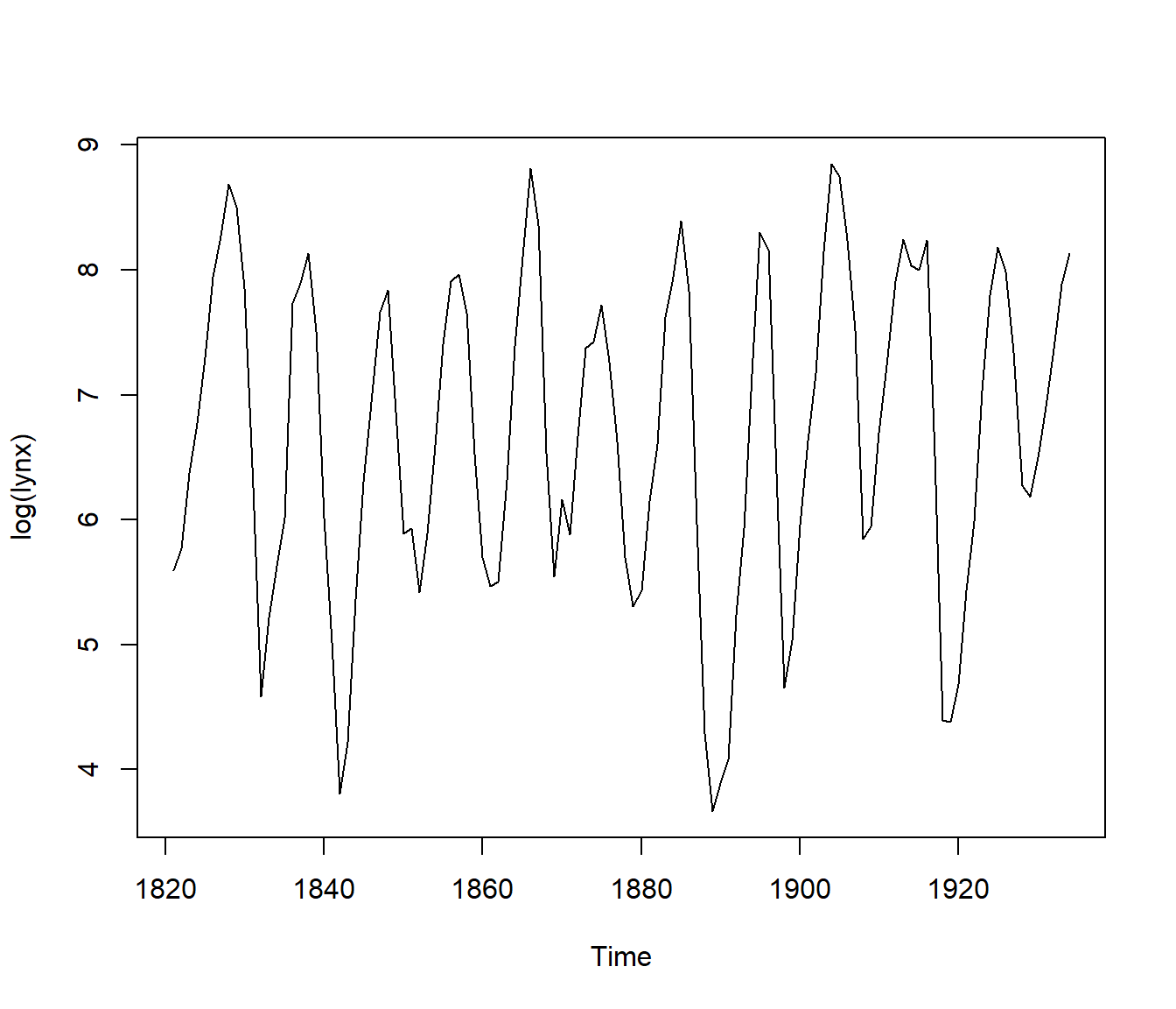
Figura 9.3: Lynx data (logarithmic scale).
lynx.ar <- ar(log(lynx))
lynx.ar$order
## [1] 11The best model is AR(11). How well determined is this, and what is the variance of the series average? We bootstrap to see, using
lynx.fun(given below), which calculates the order of the fitted autoregressive model, the series average, and saves the series itself.
Here are results for fixed-block bootstraps with block length \(l = 20\):
set.seed(DNI)
lynx.fun <- function(tsb) {
  ar.fit <- ar(tsb, order.max=25)
  c(ar.fit$order, mean(tsb), tsb)
}
lynx.1 <- tsboot(log(lynx), lynx.fun, R=99, l=20, sim="fixed")
lynx.1
ts.plot(ts(lynx.1$t[1,3:116],start=c(1821,1)),
        main="Block simulation, l=20")
boot.array(lynx.1)[1,]
table(lynx.1$t[,1])
var(lynx.1$t[,2])
qqnorm(lynx.1$t[,2]);
abline(mean(lynx.1$t[,2]),sqrt(var(lynx.1$t[,2])),lty=2)
To obtain similar results for the stationary bootstrap with mean block length \(l = 20\):
.Random.seed <- lynx.1$seed
lynx.2 <- tsboot(log(lynx), lynx.fun, ...
# lynx.2
See if the results look different from those above. Do the simulated series using blocks look like the original? Compare the estimated variances under the two resampling schemes. Try different block lengths, and see how the variances of the series average change.
For model-based resampling we need to store results from the original model:
Check the orders of the fitted models for this scheme.
For post-blackening we need to define yet another function:
Compare these results with those above, and try the post-blackened bootstrap with
sim="geom". (Sections 8.2.2, 8.2.3)’’.
Ejercicio 9.2 (Practical 8.2, Beaver data: Davison y Hinkley, 1997) Reproducir el “Practical 8.2 (Beaver data)” en Davison, A. C., y Hinkley, D. V. (1997). Bootstrap methods and their application. Cambridge university press, http://statwww.epfl.ch/davison/BMA (caché):
“The data in beaver consist of a time series of \(n = 100\) observations on the body temperature \(y_1, \ldots, y_n\) and an indicator \(x_1, \ldots, x_n\) of activity of a female beaver, Castor canadensis.
# ?beaver
plot(beaver)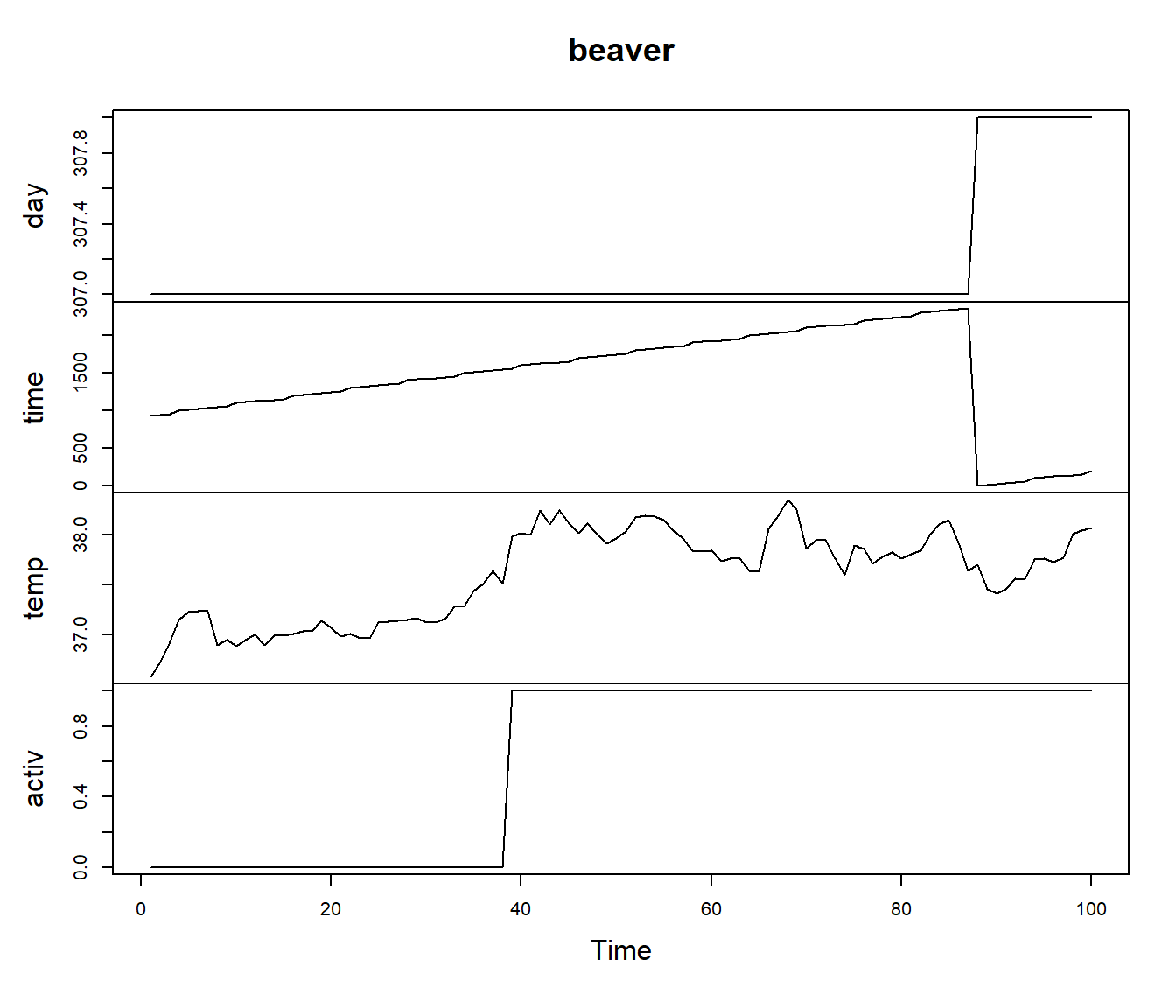
Figura 9.4: Beaver data
class(beaver)## [1] "mts" "ts"str(beaver) ## Time-Series [1:100, 1:4] from 1 to 100: 307 307 307 307 307 307 307 307 307 307 ...
## - attr(*, "dimnames")=List of 2
## ..$ : NULL
## ..$ : chr [1:4] "day" "time" "temp" "activ"We want to estimate and give an uncertainty measure for the body temperature of the beaver. The simplest model that allows for the clear autocorrelation of the series is …
To fit the original model and to generate a new series:
data <- beaver
# fit <- function( data ){
#   #  X <- cbind(rep(1,100),data$activ) # ErrorR
#   X <- cbind(rep(1, 100), data[,"activ"])
#   para <- list(X = X, data = data)
#   # assign("para",para, frame=1) # ErrorR
#   # assign("para", para, envir = .GlobalEnv)
#   para <<- para
#   # arima.mle # ErrorR
# ----------------------------
#   d <- arima.mle(x = para$data$temp,
#               model = list(ar = c(0.8)), xreg = para$X)
#   res <- arima.diag(d, plot = F, std.resid = T)$std.resid
#   res <- res[!is.na(res)]
#   list(
#     paras = c(d$model$ar, d$reg.coef, sqrt(d$sigma2)),
#     res = res - mean(res),
#     fit = X %*% d$reg.coef)
# }
#
# beaver.args <- fit(beaver)
# white.noise <- function(n.sim, ts)
#     sample(ts, size = n.sim, replace = TRUE)
# beaver.gen <- function(ts, n.sim, ran.args){
#     tsb <- ran.args$res
#     fit <- ran.args$fit
#     coeff <- ran.args$paras
#     ts$temp <- fit + coeff[4] * arima.sim(model = list(ar = coeff[1]),
#         n = n.sim, rand.gen = white.noise, ts = tsb)
#     ts
# }
# new.beaver <- beaver.gen( beaver, 100, beaver.args )
Now we are able to generate data, we can bootstrap and see the results of
beaver.bootas follows:
# beaver.fun <- function(ts) fit(ts)$paras
# beaver.boot <- tsboot( beaver, beaver.fun, R=99,sim="model",
#         n.sim=100,ran.gen=beaver.gen,ran.args=beaver.args)
# names(beaver.boot)
# beaver.boot$t0
# beaver.boot$t[1:10,]
showing the original value of
beaver.funand its value for the first 10 replicate series. Are the estimated mean temperatures for theR = 99simulations normal? Useboot.cito obtain normal and basic bootstrap confidence intervals for the resting and active temperatures. In this analysis we have assumed that the linear model with AR(1) errors is appropriate. How would you proceed if it were not? (Section 8.2; Reynolds, 1994)’’.
Ejercicio 9.3 (Practical 8.3, Sunspot data: Davison y Hinkley, 1997) Reproducir el “Practical 8.3 (Sunspot data)” en Davison, A. C., y Hinkley, D. V. (1997). Bootstrap methods and their application. Cambridge university press, http://statwww.epfl.ch/davison/BMA (caché):
“Consider scrambling the phases of the sunspot data. To see the original data,
data(sunspot.year)  # WarningR: data set 'sunspot' not found
# ?sunspot.year
yl <- c(-50, 200)
plot(sunspot.year, ylim = yl)
abline(h = 0, lty = 2)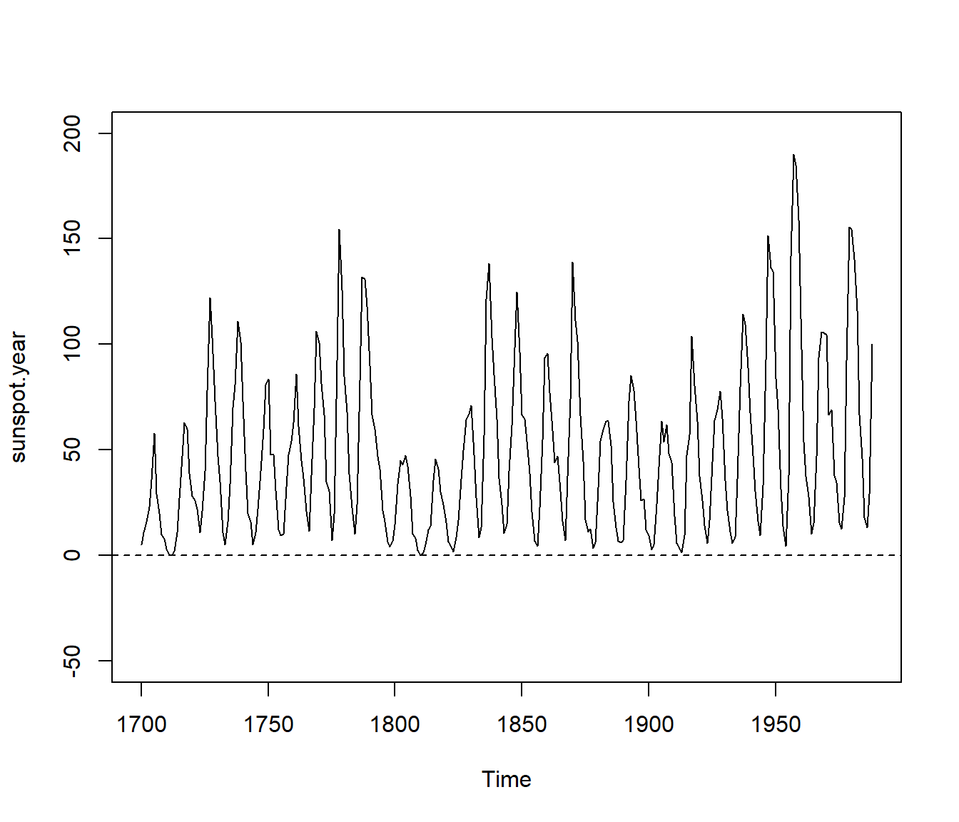
Figura 9.5: Sunspot data (yearly numbers).
two replicates generated using ordinary phase scrambling, and two phase scrambled series whose marginal distribution is the same as that of the original data:
set.seed(DNI)
sunspot.1 <- tsboot(sunspot.year, ...
.Random.seed <- sunspot.1$seed # set.seed(DNI)
sunspot.2 <- tsboot(sunspot.year, ...
What features of the original data are preserved by the two algorithms? (You may find it helpful to experiment with different shapes for the figures.) (Section 8.2.4; Problem 8.4; Theiler et al, 1992)’’.